Simulation and Prediction

Introduction

Understanding exposure-lag associations is important for epidemiological interpretation, but researchers are often interested in a different question:

What is the expected disease outcome under an alternative environmental profile?

EpiExposure provides simulation and prediction tools that allow researchers to:

generate complete synthetic exposure profiles;
introduce structured exposure events;
construct hypothetical epidemiological scenarios;
predict expected disease outcomes;
propagate parameter uncertainty;
compare alternative exposure profiles and their predictions.

Unlike lag-specific effect summaries, prediction evaluates all exposure values and lags jointly. Therefore, every prediction represents a complete environmental profile rather than an isolated exposure value.

What you will learn. This tutorial shows how to simulate complete exposure profiles, predict expected disease outcomes, propagate parameter uncertainty, construct scenario grids, and compare alternative environmental conditions.

The outputs describe predictions and contrasts under the fitted statistical model. Hypothetical scenarios should not automatically be interpreted as causal interventions unless the study design and assumptions support that interpretation.

Preparing the example model

This section uses the same dataset and DLNM specification introduced in the previous tutorials.

library(EpiExposure)
library(ggplot2)

data("epi_data")

Define the exposure-lag structures:

cb <- define_exposures(
  data = epi_data,
  vars = c(
    "tmean",
    "rain",
    "wetness"
  ),
  max_lag = 85,
  df_var = 3,
  df_lag = 2
)

Build the epidemic-level design:

dat <- build_design(
  data = epi_data,
  cb_templates = cb
)

Prepare the response:

dat <- prepare_response(
  data = dat,
  response = "y",
  family = "beta"
)

Fit the model:

fit <- fit_epidlnm(
  data = dat,
  model_engine = "glmmTMB",
  family = "beta",
  random_effect = NULL,
  epiexposure_spec = attr(
    cb,
    "spec"
  )
)

The fitted model relates complete profiles of temperature, rainfall, and leaf wetness to the expected disease response.

Complete exposure profiles

Each exposure profile supplied to predict_outcomes() must contain exactly max_lag + 1 observations. With max_lag = 85, each profile therefore contains 86 values.

Profiles are supplied in chronological order, from the earliest exposure observation to the most recent:

the first value (time = 0) is the oldest observation and corresponds to lag 85;
the final value (time = 85) is the most recent observation and corresponds to lag 0.

More generally, chronological time and retrospective lag are related by:

$\text{lag} = \text{max\_lag} - \text{time}.$

Profile construction and visualization use chronological time, whereas DLNM effects are interpreted on the retrospective lag scale. Thus, chronological time increases from the oldest to the most recent observation, while retrospective lag increases in the opposite direction, from the most recent to progressively older observations.

simulate_exposures() generates profiles directly in chronological order and does not reverse them. Simulated or manually defined profiles should therefore be supplied to predict_outcomes() in the same order in which they were created. Users should not reverse the profiles manually.

Complete profiles are required. Temperature, rainfall, and leaf wetness profiles must have the same length and temporal interpretation used to fit the model. Coordinates, blocks, years, and other grouping variables are not exposure profiles.

Simulating exposure profiles

Why simulate exposures?

Environmental conditions rarely occur as isolated observations. Disease development can reflect sequences of temperature, rainfall, leaf wetness, and other exposures occurring throughout the epidemic.

simulate_exposures() generates complete chronological profiles that can be used in prediction and scenario analysis.

A simulated exposure profile is not a disease prediction. It becomes a prediction scenario only after it is combined with the other required exposures and supplied to predict_outcomes().

Simulating a background process

The following example generates a temperature profile using an autoregressive background process:

temperature_profile <- simulate_exposures(
  max_lag = 85,
  mode = "profile",
  seed = 123,
  background = list(
    dist = "ar1",
    mean = 25,
    sd = 4,
    phi = 0.90
  )
)

The result contains the simulated chronological profile:

#>   time_0   time_1   time_2   time_3   time_4   time_5   time_6   time_7 
#> 22.75810 22.58096 25.54056 25.60944 25.77392 28.68685 29.12180 26.50391 
#>   time_8   time_9  time_10  time_11  time_12  time_13  time_14  time_15 
#> 25.15595 24.36331 26.56124 27.03248 27.52800 27.46818 26.25222 29.24259 
#>  time_16  time_17  time_18  time_19  time_20  time_21  time_22  time_23 
#> 29.68636 25.78881 26.93278 25.91517 23.96184 23.68560 22.02814 21.05446 
#>  time_24  time_25  time_26  time_27  time_28  time_29  time_30  time_31 
#> 20.35922 17.88245 20.05494 20.81686 19.25076 22.01179 23.05417 22.73428 
#>  time_32  time_33  time_34  time_35  time_36  time_37  time_38  time_39 
#> 24.52156 26.10048 27.42291 28.38130 29.00896 28.50012 27.61664 26.69160 
#>  time_40  time_41  time_42  time_43  time_44  time_45  time_46  time_47 
#> 25.31118 24.91755 22.71950 26.72925 28.66248 26.33803 25.50177 24.63795 
#>  time_48  time_49  time_50  time_51  time_52  time_53  time_54  time_55 
#> 26.03407 25.78531 26.14845 25.98383 25.81070 28.11587 27.41064 29.81363 
#>  time_56  time_57  time_58  time_59  time_60  time_61  time_62  time_63 
#> 26.63193 27.48804 27.45519 27.58617 27.98948 26.81470 26.05226 24.17109 
#>  time_64  time_65  time_66  time_67  time_68  time_69  time_70  time_71 
#> 22.38525 23.17595 24.13983 24.31826 25.99447 29.46946 28.16638 23.82356 
#>  time_72  time_73  time_74  time_75  time_76  time_77  time_78  time_79 
#> 25.69477 24.38876 23.25030 25.21342 24.69556 22.59761 23.15396 23.09640 
#>  time_80  time_81  time_82  time_83  time_84  time_85 
#> 23.29681 24.13889 23.57873 24.84437 24.47550 25.10643

The profile is ordered from the oldest to the most recent exposure observation. For this 86-value profile, the first value corresponds to lag 85 and the final value corresponds to lag 0. The profile remains in chronological order when it is later supplied to predict_outcomes().

Visualize the complete profile:


df_tmean <- data.frame(
  time = 0:85,
  value = as.numeric(temperature_profile$profile)
)

 df_tmean%>% 
  ggplot(aes(time,value))+
  geom_line(color = "#C44E52", size = 1.4)+
  theme_bw()+
  labs(x = "Days after planting the crop",
       y = "Exposure")+
  scale_x_continuous(
  limits = c(0, 85),
  breaks = seq(0, 85, by = 10)
)+
  theme(text = element_text(size = 10, face = "bold"))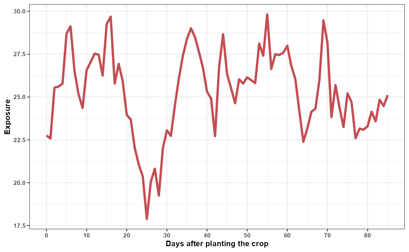

The autoregressive parameter:

phi = 0.90

produces temporal dependence among consecutive observations. It does not represent an exposure-lag effect. The lag-response relationship remains determined by the fitted DLNM.

Simulating structured exposure events

A structured event can be superimposed on a background profile.

The following example constructs a rainfall pattern with values assigned to selected portions of the temporal profile:

rain_profile <- simulate_exposures(
  max_lag = 85,
  mode = "pattern",
  pattern = "block_times",
  block_times = c(
    0,
    40
  ),
  fixed_value = 15,
  background = list(
    dist = "fixed",
    value = 0
  )
)

#>  time_0  time_1  time_2  time_3  time_4  time_5  time_6  time_7  time_8  time_9 
#>      15      15      15      15      15      15      15      15      15      15 
#> time_10 time_11 time_12 time_13 time_14 time_15 time_16 time_17 time_18 time_19 
#>      15      15      15      15      15      15      15      15      15      15 
#> time_20 time_21 time_22 time_23 time_24 time_25 time_26 time_27 time_28 time_29 
#>      15      15      15      15      15      15      15      15      15      15 
#> time_30 time_31 time_32 time_33 time_34 time_35 time_36 time_37 time_38 time_39 
#>      15      15      15      15      15      15      15      15      15      15 
#> time_40 time_41 time_42 time_43 time_44 time_45 time_46 time_47 time_48 time_49 
#>      15       0       0       0       0       0       0       0       0       0 
#> time_50 time_51 time_52 time_53 time_54 time_55 time_56 time_57 time_58 time_59 
#>       0       0       0       0       0       0       0       0       0       0 
#> time_60 time_61 time_62 time_63 time_64 time_65 time_66 time_67 time_68 time_69 
#>       0       0       0       0       0       0       0       0       0       0 
#> time_70 time_71 time_72 time_73 time_74 time_75 time_76 time_77 time_78 time_79 
#>       0       0       0       0       0       0       0       0       0       0 
#> time_80 time_81 time_82 time_83 time_84 time_85 
#>       0       0       0       0       0       0

Visualize the rainfall profile:

df_rain <- data.frame(
  time = 0:85,
  value = as.numeric(rain_profile$profile)
)

 df_rain%>% 
  ggplot(aes(time,value))+
  geom_line(color = "#4C72B0", size = 1.4)+
  theme_bw()+
  labs(x = "Days after planting the crop",
       y = "Exposure")+
  scale_x_continuous(
  limits = c(0, 85),
  breaks = seq(0, 85, by = 10)
)+
  theme(text = element_text(size = 10, face = "bold"))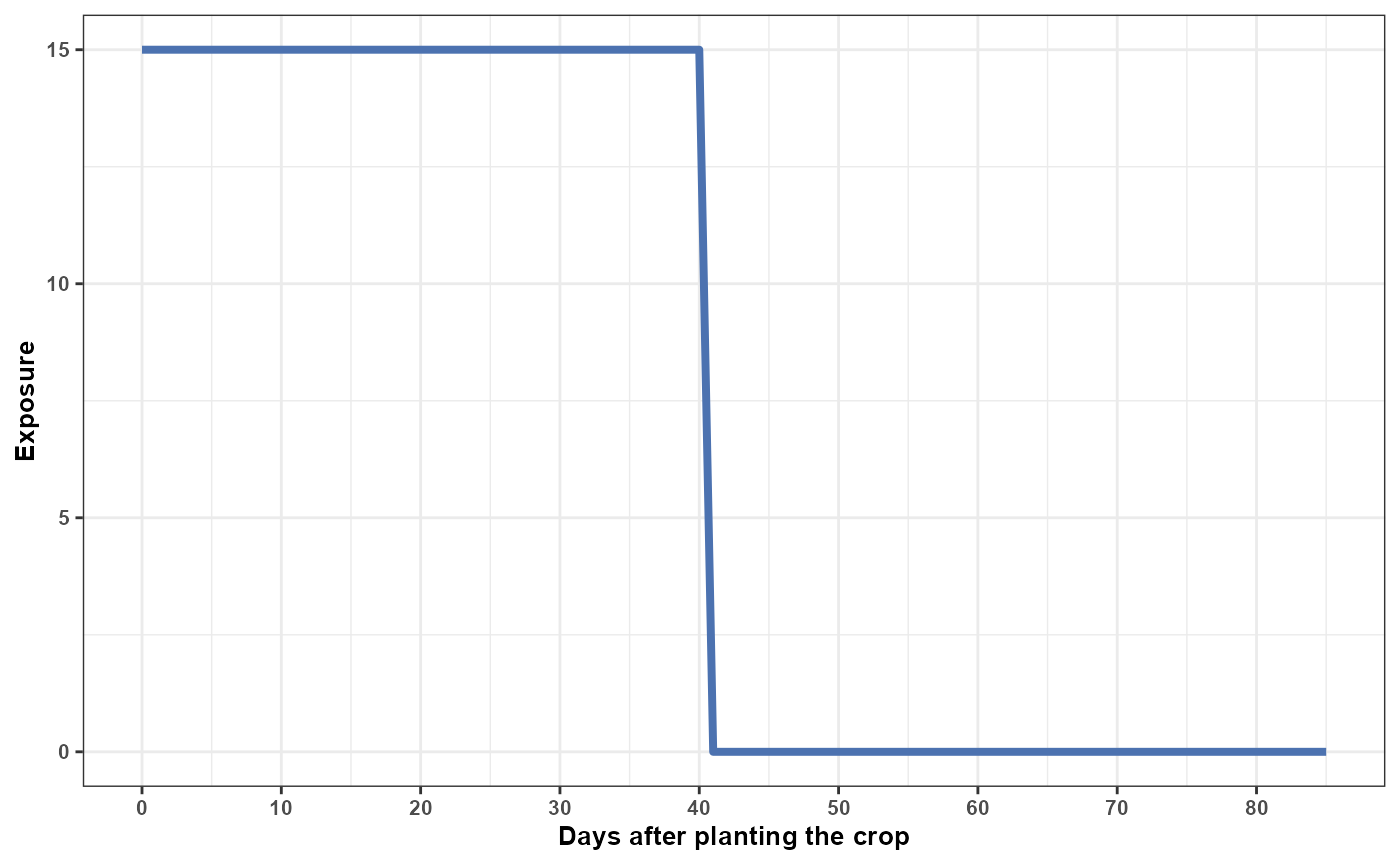

A leaf wetness profile can be generated independently:

wetness_profile <- simulate_exposures(
  max_lag = 85,
  mode = "profile",
  seed = 456,
  background = list(
    dist = "ar1",
    mean = 10,
    sd = 4,
    phi = 0.90
  )
)

#>    time_0    time_1    time_2    time_3    time_4    time_5    time_6    time_7 
#>  4.625914  6.247426  8.019056  5.795534  4.970456  4.908391  6.621729  7.396401 
#>    time_8    time_9   time_10   time_11   time_12   time_13   time_14   time_15 
#>  9.413140 10.471295  8.827395 11.230632 12.831472 15.432048 12.376714 15.534374 
#>   time_16   time_17   time_18   time_19   time_20   time_21   time_22   time_23 
#> 18.009388 17.884050 21.071020 22.645309 20.553278 16.503720 13.365585 13.392098 
#>   time_24   time_25   time_26   time_27   time_28   time_29   time_30   time_31 
#> 12.990405 14.669058 13.395137 12.483066 14.823142 12.441433 11.275305 10.112462 
#>   time_32   time_33   time_34   time_35   time_36   time_37   time_38   time_39 
#>  6.615987  7.470749  8.021169 11.384750 10.094474  9.840489  9.117208  9.137949 
#>   time_40   time_41   time_42   time_43   time_44   time_45   time_46   time_47 
#>  9.173692  9.941607  9.512229  9.706507 13.360498 13.235160 13.117645 14.148516 
#>   time_48   time_49   time_50   time_51   time_52   time_53   time_54   time_55 
#> 11.684280 12.229035 10.846750 10.314809 11.466825 12.883845 13.673602 14.581575 
#>   time_56   time_57   time_58   time_59   time_60   time_61   time_62   time_63 
#> 13.403023 15.778860 16.145459 16.537209 11.952268 10.044761  9.690582 11.283632 
#>   time_64   time_65   time_66   time_67   time_68   time_69   time_70   time_71 
#> 11.079345 13.843590 16.184937 13.070750 11.814142 10.288002  9.962817  9.895465 
#>   time_72   time_73   time_74   time_75   time_76   time_77   time_78   time_79 
#>  6.906054  9.733334  9.725104 10.223759 10.004476  8.513481  6.859744  7.560886 
#>   time_80   time_81   time_82   time_83   time_84   time_85 
#>  5.922656  5.560829  9.527843  9.702088 10.967745 12.353884

df_wetness <- data.frame(
  time = 0:85,
  value = as.numeric(wetness_profile$profile)
)


 df_wetness%>% 
  ggplot(aes(time,value))+
  geom_line(color = "#55A868", size = 1.4)+
  theme_bw()+
  labs(x = "Days after planting the crop",
       y = "Exposure")+
  scale_x_continuous(
  limits = c(0, 85),
  breaks = seq(0, 85, by = 10)
)+
  theme(text = element_text(size = 10, face = "bold"))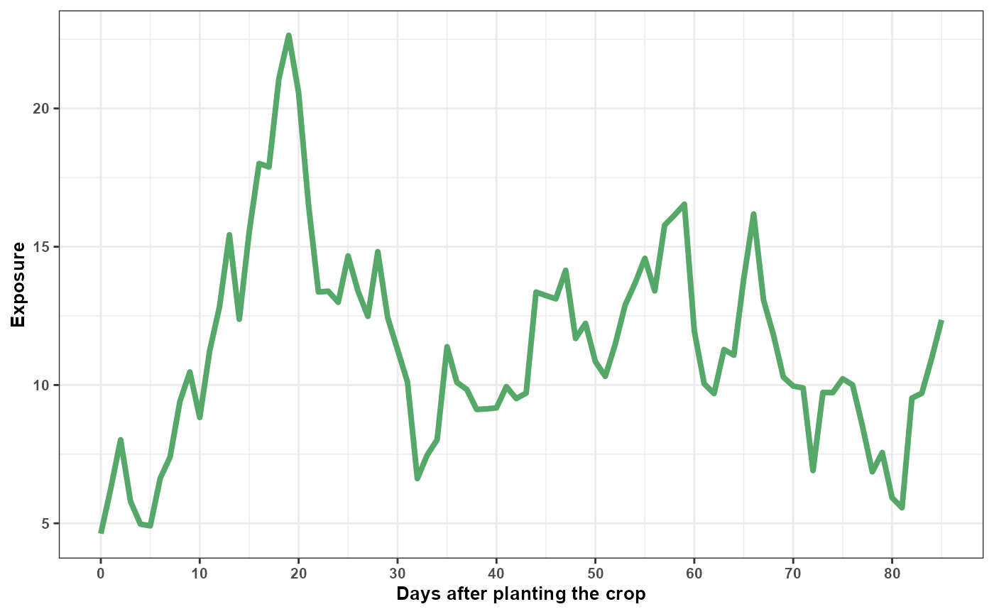

The three profiles can now be combined into one complete hypothetical environmental profile.

All three profiles follow the same chronological convention and contain 86 observations. At each chronological position, the temperature, rainfall, and leaf wetness values describe the environmental conditions assigned to that point in the hypothetical profile.

When these profiles are supplied to predict_outcomes(), the function validates their length and order and projects each complete profile through the cross-basis definition stored in the fitted model. The resulting design follows the retrospective DLNM lag convention, in which lag 0 represents the most recent exposure and increasing lags represent progressively older exposures.

This internal transformation does not require the user to reverse or otherwise rearrange the simulated profiles.

Predicting disease outcomes

Deterministic prediction

predict_outcomes() receives the complete profiles in chronological order and projects them through the cross-basis definition stored in the fitted model. The reconstructed cross-basis predictors represent the exposure profiles on the retrospective DLNM lag scale, allowing the function to calculate the population-level expected response associated with the complete multivariable profile.

prediction <- predict_outcomes(
  fit = fit,
  profiles = list(
    tmean = temperature_profile$profile,
    rain = rain_profile$profile,
    wetness = wetness_profile$profile
  ),
  uncertainty = FALSE
)

prediction
#>   prediction
#> 1  0.1195241

The prediction combines:

the complete chronological temperature profile;
the complete chronological rainfall profile;
the complete chronological leaf wetness profile;
the corresponding retrospective lag contributions reconstructed from the fitted cross-basis;
the fitted joint cross-basis coefficients;
the inverse link required by the response family.

The output represents one joint prediction for the three complete exposure profiles. It is not calculated independently for each day or lag.

The prediction is not a newly simulated disease observation. It represents the central expected response associated with the complete exposure profile.

For the fitted Beta model, the result is an expected response on the proportion scale.

Prediction uncertainty

A deterministic prediction uses the central fitted coefficient estimates. However, the coefficients are estimated with uncertainty.

When:

uncertainty = TRUE

EpiExposure propagates joint coefficient uncertainty through the complete prediction calculation.

To inspect individual uncertainty realizations, request sample-level output:

prediction_samples <- predict_outcomes(
  fit = fit,
  profiles = list(
    tmean = temperature_profile$profile,
    rain = rain_profile$profile,
    wetness = wetness_profile$profile
  ),
  uncertainty = TRUE,
  n_samples = 100,
  output = "samples",
  seed = 123
)

head(prediction_samples)
#>   sample prediction
#> 1      1  0.1034903
#> 2      2  0.1042327
#> 3      3  0.0892574
#> 4      4  0.1337358
#> 5      5  0.0837315
#> 6      6  0.1593514

Inspect the first realizations:

sample	prediction
1	0.1035
2	0.1042
3	0.0893
4	0.1337
5	0.0837
6	0.1594
7	0.1302
8	0.2368
9	0.1578
10	0.1566

Visualize the prediction distribution:

ggplot(
  prediction_samples,
  aes(
    x = prediction * 100
  )
) +
  geom_histogram(
    bins = 25,
    fill = "#4C72B0",
    color = "white"
  ) +
  theme_bw() +
  labs(
    x = "Predicted disease response (%)",
    y = "Number of uncertainty realizations",
    title = "Parameter uncertainty in the predicted response"
  )

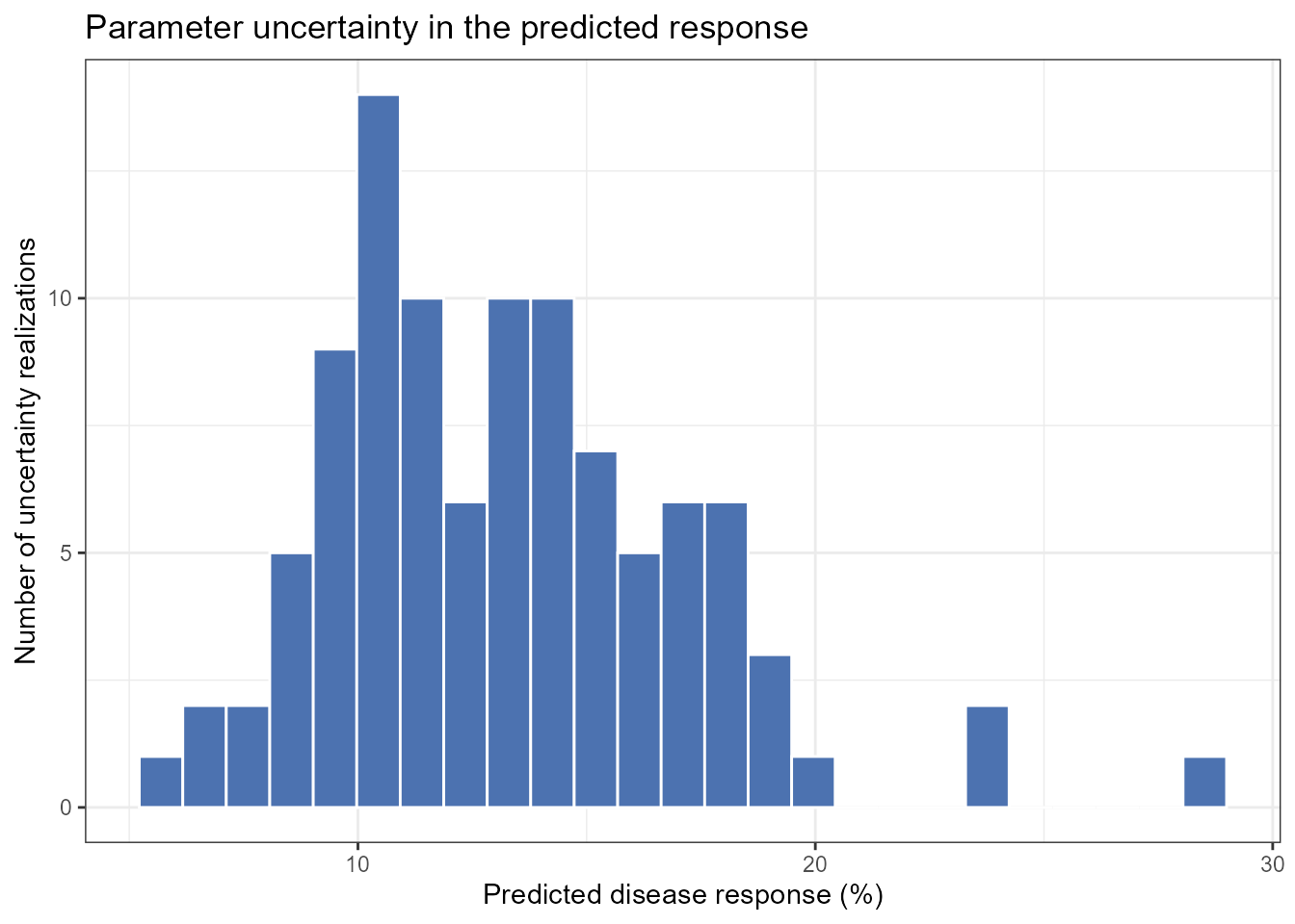
This distribution represents parameter uncertainty in the expected response. It does not include observation-level noise and should not be interpreted as a distribution of newly simulated disease observations.

A summarized prediction can also be requested when individual realizations are not needed:

prediction_summary <- predict_outcomes(
  fit = fit,
  profiles = list(
    tmean = temperature_profile$profile,
    rain = rain_profile$profile,
    wetness = wetness_profile$profile
  ),
  uncertainty = TRUE,
  n_samples = 100,
  output = "summary",
  seed = 123
)

prediction_summary
#>   prediction prediction_sd prediction_lower prediction_upper
#> 1  0.1293006    0.03879026       0.07271773        0.2212469

Scenario simulation

Why construct scenarios?

A single profile describes one complete hypothetical profile. Scenario analysis extends this idea by evaluating multiple combinations of environmental conditions systematically.

Possible questions include:

How does the predicted response change across rainfall levels?
Does the rainfall association differ under distinct temperature conditions?
Which combinations of temperature and leaf wetness yield larger expected responses?
How does the timing of an exposure pattern alter the prediction?

These are model-based comparisons. They describe how the fitted model responds to supplied profiles and do not automatically demonstrate causal interventions.

Defining epidemiological periods

The scenario grid can be organized using epidemiological periods:

periods <- define_periods(
  max_lag = 85,
  cuts = c(
    20,
    40,
    60
  ),
  prefix = "Period"
)

periods
#>    period lag_start lag_end
#> 1 Period1         0      20
#> 2 Period2        21      40
#> 3 Period3        41      60
#> 4 Period4        61      85

The resulting periods divide the retrospective lag interval into four subintervals.

Remember that lag order is retrospective:

smaller lag → closer to disease assessment
larger lag  → earlier exposure condition

Generating candidate scenarios

The following example varies rainfall across a grid while evaluating selected temperature and leaf wetness conditions:

scenarios <- simulate_ranges(
  periods = periods,
  vary = list(
    tmean = c(
      20,
      34
    ),
    rain = seq(
      0,
      15,
      by = 1
    ),
    wetness = c(
      2,
      10
    )
  ),
  scenario_type = "grid",
  scenario_var = "rain"
)

Predicting scenario outcomes

simulate_scenarios() evaluates the expected disease outcome associated with each complete exposure scenario. When uncertainty = TRUE, uncertainty in the joint fitted model parameters is propagated through the prediction calculation.

Summarizing scenario predictions

With:

output = "summary"

the parameter-draw predictions are summarized for each scenario. The prediction column contains the median expected response across the parameter draws, while prediction_lower and prediction_upper contain the empirical uncertainty interval defined by the selected probabilities. The default probabilities correspond to a 95% interval.

pred_scenarios <- simulate_scenarios(
  fit = fit,
  scenarios = scenarios,
  data = epi_data,
  uncertainty = TRUE,
  output = "summary",
  n_samples = 100,
  seed = 123
)

Inspect the summarized predictions:

scenario	scenario_point	tmean	rain	wetness	prediction	prediction_sd	prediction_lower	prediction_upper
RAIN_s1	1	20	0	2	0.0066	0.0022	0.0039	0.0119
RAIN_s2	1	34	0	2	0.0015	0.0018	0.0003	0.0063
RAIN_s3	1	20	1	2	0.0326	0.0339	0.0107	0.1403
RAIN_s4	1	34	1	2	0.0067	0.0226	0.0016	0.0880
RAIN_s5	1	20	2	2	0.0591	0.0432	0.0211	0.1866
RAIN_s6	1	34	2	2	0.0117	0.0318	0.0031	0.1212
RAIN_s7	1	20	3	2	0.0943	0.0472	0.0398	0.2148
RAIN_s8	1	34	3	2	0.0206	0.0396	0.0052	0.1504
RAIN_s9	1	20	4	2	0.1443	0.0514	0.0696	0.2589
RAIN_s10	1	34	4	2	0.0314	0.0499	0.0088	0.1844

Visualizing summarized scenario predictions

The modeled rainfall association can be displayed across the selected combinations of temperature and leaf wetness. For summary output, plot_scenarios() displays the central predicted response together with the corresponding lower and upper uncertainty limits.

plot_scenarios(
  data = pred_scenarios,
  x = "rain",
  facet = c(
    "wetness",
    "tmean"
  ),
  x_limits = c(
    0,
    15
  ),
  output = "summary"
)

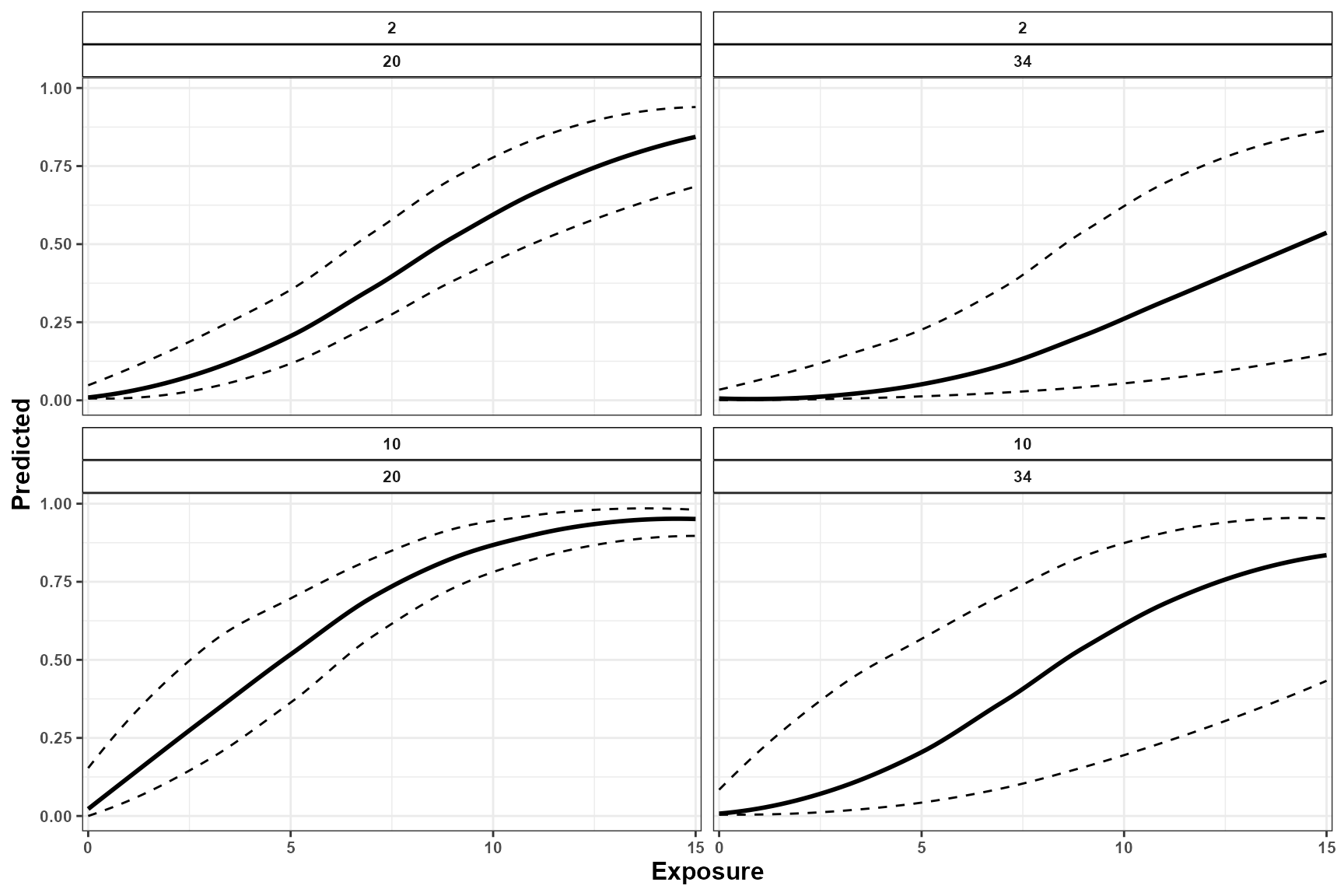
The central curve represents the median expected response for each scenario, whereas the lower and upper curves describe uncertainty arising from the fitted model parameters.

Returning individual prediction samples

With:

output = "samples"

simulate_scenarios() returns every draw-specific prediction instead of summarizing the draws. Each row represents one parameter draw for one scenario in the exposure grid.

These samples are not additional exposure simulations and are not newly simulated disease observations. The exposure scenarios remain fixed; what changes across samples is the joint draw of the fitted model parameters used to calculate the expected response.

Draw-level output is useful for constructing customized uncertainty summaries, examining the complete distribution of expected responses, propagating parameter uncertainty into downstream calculations, or creating custom visualizations.

pred_scenarios_s <- simulate_scenarios(
  fit = fit,
  scenarios = scenarios,
  data = epi_data,
  uncertainty = TRUE,
  output = "samples",
  n_samples = 100,
  seed = 123
)

Inspect the first draw-specific predictions:

scenario	scenario_point	tmean	wetness	sample	prediction
RAIN_s1	1	20	2	1	0.0067
RAIN_s1	1	20	2	2	0.0070
RAIN_s1	1	20	2	3	0.0099
RAIN_s1	1	20	2	4	0.0062
RAIN_s1	1	20	2	5	0.0056
RAIN_s1	1	20	2	6	0.0120
RAIN_s1	1	20	2	7	0.0050
RAIN_s1	1	20	2	8	0.0050
RAIN_s1	1	20	2	9	0.0046
RAIN_s1	1	20	2	10	0.0047

Visualizing individual prediction samples

When draw-level output is supplied, plot_scenarios() displays the prediction curves associated with the individual parameter draws. The collection of curves shows how uncertainty in the fitted parameters propagates across the complete scenario grid.

plot_scenarios(
  data = pred_scenarios_s,
  x = "rain",
  facet = c(
    "wetness",
    "tmean"
  ),
  x_limits = c(
    0,
    15
  ),
  output = "samples"
)

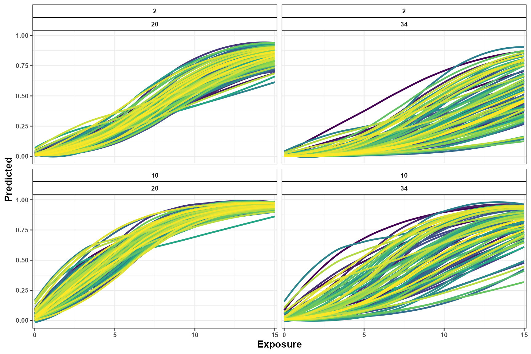
The summary and sample outputs describe the same parameter-uncertainty distribution at different levels of detail:

output = "summary" reports the median expected response and its empirical uncertainty interval for each scenario;
output = "samples" retains every draw-specific expected response used to construct those summaries.

The figures should be interpreted as visualizations of the fitted model over the scenario grid. Predictions outside or near the limits of the observed exposure support should be treated cautiously. Neither output includes observation-level noise, and neither should be interpreted as a distribution of newly simulated disease observations.

Scenario surfaces

When enough values are evaluated along two continuous dimensions, predictions can be presented as a scenario surface.

The current example evaluates only two temperature values. Therefore, a line or point representation is more appropriate than a dense continuous surface.

A tile display can still summarize the evaluated grid:

ggplot(
  pred_scenarios,
  aes(
    x = rain,
    y = factor(
      tmean
    ),
    fill = prediction * 100
  )
) +
  geom_tile() +
  facet_wrap(
    vars(
      wetness
    ),
    labeller = label_both
  ) +
  scale_fill_viridis_c(
    name = "Expected\ndisease (%)"
  ) +
  theme_bw() +
  labs(
    x = "Rainfall",
    y = "Mean temperature",
    title = "Predicted response across the evaluated scenario grid"
  )

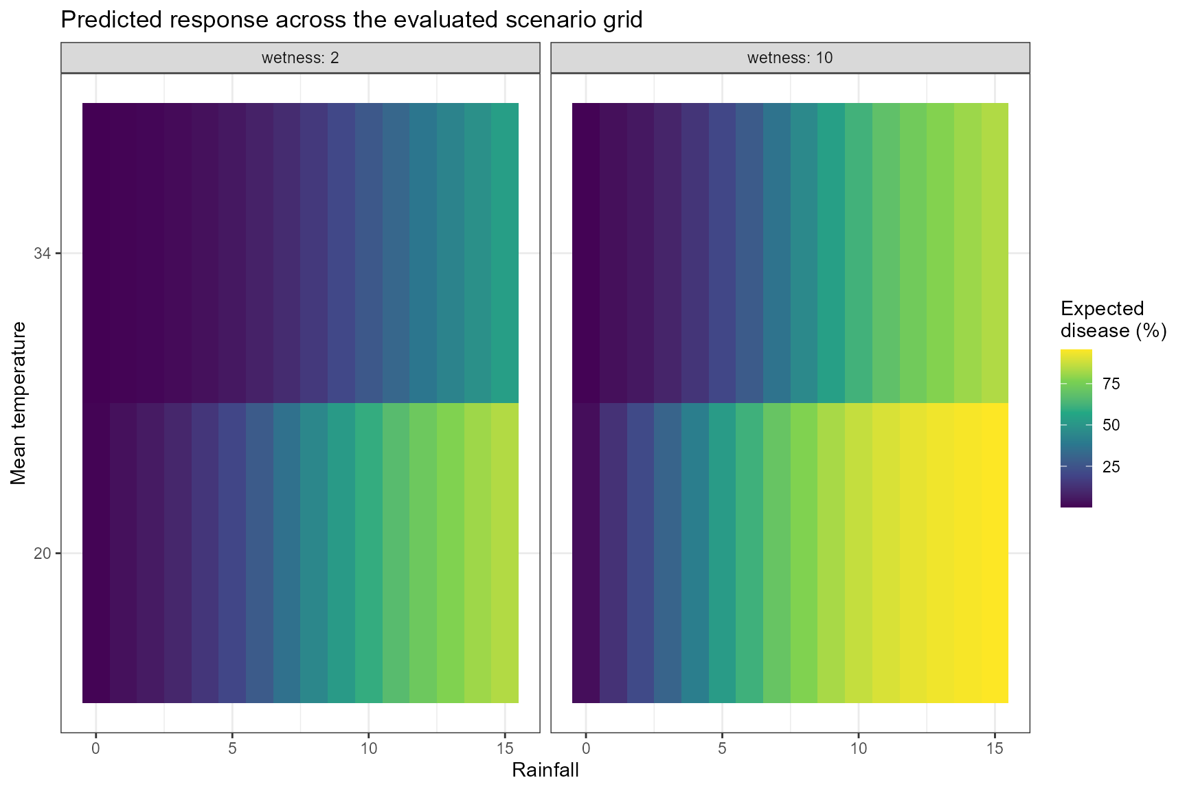
A smoother surface requires a denser sequence of temperature values in simulate_ranges().

Comparing predictions

Comparing complete simulated profiles

A single prediction describes the expected response associated with one complete environmental profile. compare_predictions() extends this analysis by contrasting the expected responses associated with two or more complete profiles.

The following example constructs four hypothetical environmental scenarios. Each scenario contains chronological temperature, rainfall, and leaf wetness profiles generated with autoregressive background processes.

The scenarios differ in their mean exposure values, temporal variability, and persistence:

Scenario A: moderate temperature and rainfall with prolonged leaf wetness;
Scenario B: high temperature, moderate rainfall, and low leaf wetness;
Scenario C: cool and relatively dry conditions with low leaf wetness;
Scenario D: cooler conditions with high rainfall and prolonged leaf wetness.

Because several exposures differ simultaneously, the resulting prediction contrasts represent joint differences between the complete environmental profiles. They should not be attributed to one exposure individually.

Defining Scenario A

exposure_tmean_A <- simulate_exposures(
  max_lag = 85,
  mode = "profile",
  seed = 101,
  background = list(
    dist = "ar1",
    mean = 25,
    sd = 2,
    phi = 0.90
  ),
  n = 1
)

exposure_rain_A <- simulate_exposures(
  max_lag = 85,
  mode = "profile",
  seed = 102,
  background = list(
    dist = "ar1",
    mean = 5,
    sd = 2,
    phi = 0.50
  ),
  n = 1
)

exposure_wetness_A <- simulate_exposures(
  max_lag = 85,
  mode = "profile",
  seed = 103,
  background = list(
    dist = "ar1",
    mean = 15,
    sd = 3,
    phi = 0.70
  ),
  n = 1
)

scenario_A <- list(
  tmean = exposure_tmean_A,
  rain = exposure_rain_A,
  wetness = exposure_wetness_A
)

Defining Scenario B

exposure_tmean_B <- simulate_exposures(
  max_lag = 85,
  mode = "profile",
  seed = 201,
  background = list(
    dist = "ar1",
    mean = 34,
    sd = 2,
    phi = 0.95
  ),
  n = 1
)

exposure_rain_B <- simulate_exposures(
  max_lag = 85,
  mode = "profile",
  seed = 202,
  background = list(
    dist = "ar1",
    mean = 5,
    sd = 1.5,
    phi = 0.40
  ),
  n = 1
)

exposure_wetness_B <- simulate_exposures(
  max_lag = 85,
  mode = "profile",
  seed = 203,
  background = list(
    dist = "ar1",
    mean = 2,
    sd = 0.7,
    phi = 0.60
  ),
  n = 1
)

scenario_B <- list(
  tmean = exposure_tmean_B,
  rain = exposure_rain_B,
  wetness = exposure_wetness_B
)

Defining Scenario C

exposure_tmean_C <- simulate_exposures(
  max_lag = 85,
  mode = "profile",
  seed = 301,
  background = list(
    dist = "ar1",
    mean = 15,
    sd = 2,
    phi = 0.90
  ),
  n = 1
)

exposure_rain_C <- simulate_exposures(
  max_lag = 85,
  mode = "profile",
  seed = 302,
  background = list(
    dist = "ar1",
    mean = 0.5,
    sd = 0.5,
    phi = 0.40
  ),
  n = 1
)

exposure_wetness_C <- simulate_exposures(
  max_lag = 85,
  mode = "profile",
  seed = 303,
  background = list(
    dist = "ar1",
    mean = 2,
    sd = 0.8,
    phi = 0.60
  ),
  n = 1
)

scenario_C <- list(
  tmean = exposure_tmean_C,
  rain = exposure_rain_C,
  wetness = exposure_wetness_C
)

Defining Scenario D

exposure_tmean_D <- simulate_exposures(
  max_lag = 85,
  mode = "profile",
  seed = 401,
  background = list(
    dist = "ar1",
    mean = 10,
    sd = 2,
    phi = 0.90
  ),
  n = 1
)

exposure_rain_D <- simulate_exposures(
  max_lag = 85,
  mode = "profile",
  seed = 402,
  background = list(
    dist = "ar1",
    mean = 15,
    sd = 4,
    phi = 0.60
  ),
  n = 1
)

exposure_wetness_D <- simulate_exposures(
  max_lag = 85,
  mode = "profile",
  seed = 403,
  background = list(
    dist = "ar1",
    mean = 20,
    sd = 3,
    phi = 0.70
  ),
  n = 1
)

scenario_D <- list(
  tmean = exposure_tmean_D,
  rain = exposure_rain_D,
  wetness = exposure_wetness_D
)

All profiles contain 86 observations and are ordered chronologically from the oldest to the most recent exposure. The profiles should not be reversed before being supplied to compare_predictions().

Visualizing the candidate profiles

Before comparing their predicted outcomes, the complete exposure profiles can be inspected to verify how the scenarios differ.

The following helper converts one simulated exposure profile into a data frame:

profile_to_data <- function(
    exposure,
    variable,
    scenario
) {
  data.frame(
    scenario = scenario,
    var = variable,
    time = 0:85,
    lag = 85:0,
    value = as.numeric(exposure$profile),
    stringsAsFactors = FALSE
  )
}

df_simulations <- dplyr::bind_rows(
  profile_to_data(
    exposure_tmean_A,
    variable = "tmean",
    scenario = "A"
  ),
  profile_to_data(
    exposure_rain_A,
    variable = "rain",
    scenario = "A"
  ),
  profile_to_data(
    exposure_wetness_A,
    variable = "wetness",
    scenario = "A"
  ),
  profile_to_data(
    exposure_tmean_B,
    variable = "tmean",
    scenario = "B"
  ),
  profile_to_data(
    exposure_rain_B,
    variable = "rain",
    scenario = "B"
  ),
  profile_to_data(
    exposure_wetness_B,
    variable = "wetness",
    scenario = "B"
  ),
  profile_to_data(
    exposure_tmean_C,
    variable = "tmean",
    scenario = "C"
  ),
  profile_to_data(
    exposure_rain_C,
    variable = "rain",
    scenario = "C"
  ),
  profile_to_data(
    exposure_wetness_C,
    variable = "wetness",
    scenario = "C"
  ),
  profile_to_data(
    exposure_tmean_D,
    variable = "tmean",
    scenario = "D"
  ),
  profile_to_data(
    exposure_rain_D,
    variable = "rain",
    scenario = "D"
  ),
  profile_to_data(
    exposure_wetness_D,
    variable = "wetness",
    scenario = "D"
  )
)

Although both chronological time and retrospective lag are retained in df_simulations, the profiles are visualized below in chronological order. Thus, time 0 is the oldest observation and time 85 is the most recent observation.

simulation_plot <- ggplot(
  df_simulations,
  aes(
    x = time,
    y = value,
    color = var
  )
) +
  geom_line(linewidth = 1) +
  facet_grid(
    rows = vars(var),
    cols = vars(scenario),
    scales = "free_y"
  ) +
  scale_x_continuous(
    limits = c(
      0,
      85
    ),
    breaks = seq(
      0,
      85,
      by = 15
    )
  ) +
  scale_color_manual(
    values = c(
      tmean = "#C44E52",
      rain = "#4C72B0",
      wetness = "#55A868"
    )
  ) +
  theme_bw() +
  labs(
    x = "Chronological time",
    y = "Exposure",
    color = "Variable"
  ) +
  theme(
    text = element_text(
      size = 10,
      face = "bold"
    ),
    legend.position = "none",
    strip.background = element_rect(
      color = "black",
      fill = "white"
    ),
    strip.text = element_text(
      face = "bold"
    )
  )

simulation_plot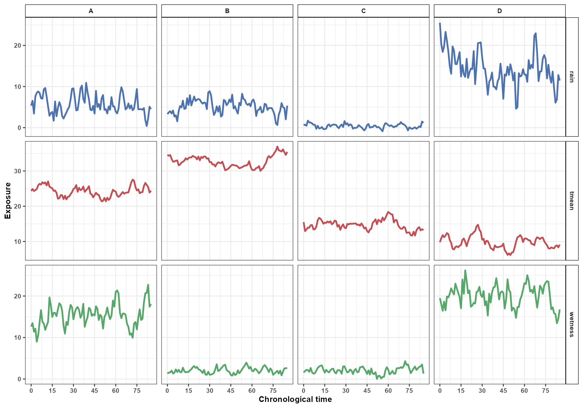

The figure shows the exposure profiles exactly as they are supplied to compare_predictions(). Internally, EpiExposure projects each chronological profile through the fitted cross-basis, where lag 0 represents the most recent exposure and increasing lags represent progressively older exposures.

Comparing the exposure profiles

Before comparing the predicted disease outcomes, the exposure profiles themselves can be compared directly.

compare_exposures() describes how two chronological exposure profiles differ across time. This comparison does not use the fitted disease model and does not produce a predicted response. It only quantifies differences between the supplied exposure profiles.

The following example compares Scenarios A and D. These scenarios differ in temperature, rainfall, and leaf wetness, so each exposure is compared separately.

Comparing temperature profiles

comparison_tmean_AD <- compare_exposures(
  exposure1 = exposure_tmean_A$profile,
  exposure2 = exposure_tmean_D$profile,
  mode = "timewise"
)

comparison_tmean_AD$var <- "tmean"
comparison_tmean_AD$scenario1 <- "A"
comparison_tmean_AD$scenario2 <- "D"

Comparing rainfall profiles

comparison_rain_AD <- compare_exposures(
  exposure1 = exposure_rain_A$profile,
  exposure2 = exposure_rain_D$profile,
  mode = "timewise"
)

comparison_rain_AD$var <- "rain"
comparison_rain_AD$scenario1 <- "A"
comparison_rain_AD$scenario2 <- "D"

Comparing leaf wetness profiles

comparison_wetness_AD <- compare_exposures(
  exposure1 = exposure_wetness_A$profile,
  exposure2 = exposure_wetness_D$profile,
  mode = "timewise"
)

comparison_wetness_AD$var <- "wetness"
comparison_wetness_AD$scenario1 <- "A"
comparison_wetness_AD$scenario2 <- "D"

The three comparisons can be combined into one data frame:

exposure_comparison_AD <- dplyr::bind_rows(
  comparison_tmean_AD,
  comparison_rain_AD,
  comparison_wetness_AD
)

exposure_comparison_AD$var <- factor(
  exposure_comparison_AD$var,
  levels = c(
    "tmean",
    "rain",
    "wetness"
  )
)

Inspect the first time-specific differences:

exposure1	exposure2	position	time	lag	value1	value2	diff	abs_diff	ratio	ratio_defined	var	scenario1	scenario2
exposure1	exposure2	1	0	85	24.348	9.808	14.540	14.540	2.482	TRUE	tmean	A	D
exposure1	exposure2	2	1	84	24.895	10.920	13.975	13.975	2.280	TRUE	tmean	A	D
exposure1	exposure2	3	2	83	24.317	11.809	12.508	12.508	2.059	TRUE	tmean	A	D
exposure1	exposure2	4	3	82	24.572	11.225	13.347	13.347	2.189	TRUE	tmean	A	D
exposure1	exposure2	5	4	81	24.886	11.670	13.215	13.215	2.132	TRUE	tmean	A	D
exposure1	exposure2	6	5	80	25.921	12.378	13.542	13.542	2.094	TRUE	tmean	A	D
exposure1	exposure2	7	6	79	26.368	12.086	14.282	14.282	2.182	TRUE	tmean	A	D
exposure1	exposure2	8	7	78	26.133	10.431	15.702	15.702	2.505	TRUE	tmean	A	D
exposure1	exposure2	9	8	77	26.819	9.636	17.183	17.183	2.783	TRUE	tmean	A	D
exposure1	exposure2	10	9	76	26.443	7.942	18.501	18.501	3.330	TRUE	tmean	A	D
exposure1	exposure2	11	10	75	26.757	7.726	19.032	19.032	3.463	TRUE	tmean	A	D
exposure1	exposure2	12	11	74	25.889	8.438	17.451	17.451	3.068	TRUE	tmean	A	D

Visualizing the exposure differences

The time-specific differences can be displayed separately for each exposure:

exposure_comparison_plot <- ggplot(
  exposure_comparison_AD,
  aes(
    x = time,
    y = diff,
    color = var
  )
) +
  geom_hline(
    yintercept = 0,
    color = "grey50",
    linetype = "dashed",
    linewidth = 0.5
  ) +
  geom_line(
    linewidth = 1
  ) +
  facet_wrap(
    vars(var),
    ncol = 1,
    scales = "free_y",
    labeller = as_labeller(
      c(
        tmean = "Mean temperature",
        rain = "Rainfall",
        wetness = "Leaf wetness"
      )
    )
  ) +
  scale_x_continuous(
    limits = c(
      0,
      85
    ),
    breaks = seq(
      0,
      85,
      by = 15
    )
  ) +
  scale_color_manual(
    values = c(
      tmean = "#C44E52",
      rain = "#4C72B0",
      wetness = "#55A868"
    )
  ) +
  theme_bw() +
  labs(
    x = "Days after planting the crop",
    y = "Scenario D - Scenario A",
    color = "Exposure"
  ) +
  theme(
    text = element_text(
      size = 10,
      face = "bold"
    ),
    legend.position = "none",
    strip.background = element_rect(
      fill = "white",
      color = "black"
    ),
    strip.text = element_text(
      face = "bold"
    )
  )

exposure_comparison_plot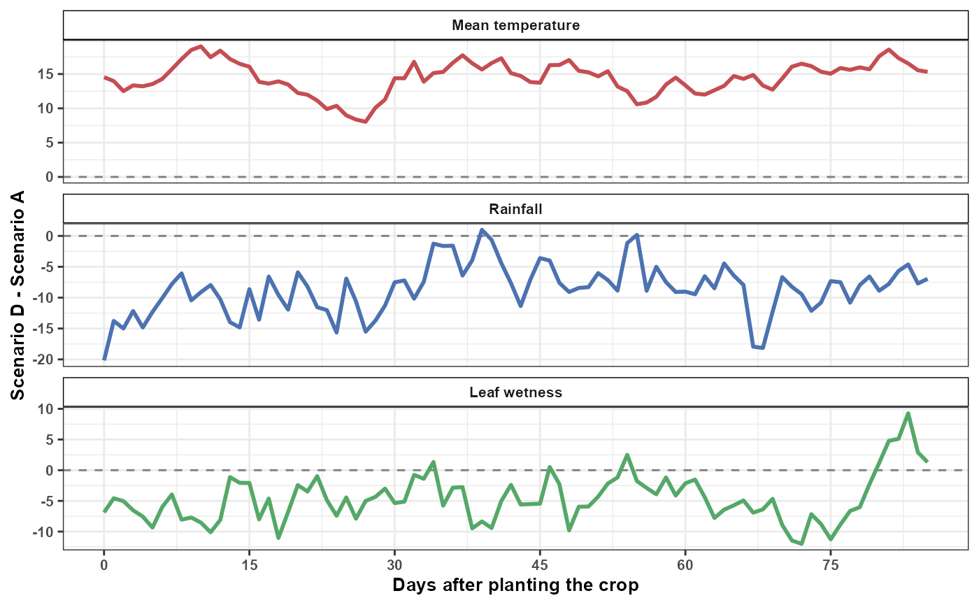

The horizontal zero line represents identical exposure values in Scenarios A and D at a given chronological time. Under the difference convention returned by compare_exposures():

positive values indicate that the exposure is higher in Scenario D than in Scenario A;
negative values indicate that the exposure is lower in Scenario D than in Scenario A;
values near zero indicate similar exposure values at that chronological position.

The facets use independent y-axis scales because temperature, rainfall, and leaf wetness are measured in different units. Consequently, the numerical magnitudes of the differences should not be compared directly across exposures.

These comparisons describe the environmental profiles themselves. They do not account for the fitted cross-basis coefficients and do not indicate how strongly each exposure difference contributes to the disease response.

The next section uses compare_predictions() to determine how the fitted model translates the complete multivariable profiles into differences in expected disease outcomes.

Comparing the expected outcomes

With four scenarios, compare_predictions() returns all pairwise comparisons:

A versus B;
A versus C;
A versus D;
B versus C;
B versus D;
C versus D.

The same joint parameter draw is used for both scenarios in each comparison. This preserves the covariance between their predictions when calculating differences, ratios, and relative changes.

Summarized comparisons

With:

output = "summary"

the function summarizes the draw-specific comparisons using their central values and empirical uncertainty intervals.

comp_pred <- compare_predictions(
  fit = fit,
  profiles = list(
    A = scenario_A,
    B = scenario_B,
    C = scenario_C,
    D = scenario_D
  ),
  uncertainty = TRUE,
  output = "summary",
  n_samples = 100,
  seed = 123
)

comp_pred <- comp_pred |>
  dplyr::mutate(
    comparison = paste(
      scenario1,
      scenario2,
      sep = " vs. "
    )
  )

Inspect selected comparison results:

comparison	pred1	pred1_lower	pred1_upper	pred2	pred2_lower	pred2_upper	diff	diff_lower	diff_upper	percentage_point_change	percentage_point_change_lower	percentage_point_change_upper
A vs. B	0.9579	0.9420	0.9714	0.1157	0.0391	0.3447	-0.8343	-0.9182	-0.6255	-83.4328	-91.8209	-62.5461
A vs. C	0.9579	0.9420	0.9714	0.0354	0.0061	0.1601	-0.9200	-0.9560	-0.7921	-92.0031	-95.5952	-79.2087
A vs. D	0.9579	0.9420	0.9714	0.9997	0.9944	1.0000	0.0416	0.0243	0.0577	4.1587	2.4322	5.7701
B vs. C	0.1157	0.0391	0.3447	0.0354	0.0061	0.1601	-0.0706	-0.2953	0.0206	-7.0565	-29.5259	2.0589
B vs. D	0.1157	0.0391	0.3447	0.9997	0.9944	1.0000	0.8839	0.6510	0.9591	88.3883	65.1010	95.9142
C vs. D	0.0354	0.0061	0.1601	0.9997	0.9944	1.0000	0.9639	0.8399	0.9898	96.3927	83.9893	98.9832

Each row compares the expected response under two complete environmental profiles. For example, diff represents the draw-by-draw difference between the expected response for scenario2 and the expected response for scenario1, summarized across the joint parameter draws.

For a Beta or Binomial response, percentage_point_change expresses the absolute change in the expected proportion or probability multiplied by 100. It is different from percent_change, which describes the relative change between predictions when that ratio is defined.

The example uses 100 parameter draws to limit the computational time required to build the tutorial. A larger number of draws may be used in a final analysis when more stable uncertainty summaries are required.

Draw-specific comparisons

With:

output = "samples"

the function retains every draw-specific comparison instead of reducing the draws to summary statistics.

comp_pred_samples <- compare_predictions(
  fit = fit,
  profiles = list(
    A = scenario_A,
    B = scenario_B,
    C = scenario_C,
    D = scenario_D
  ),
  uncertainty = TRUE,
  output = "samples",
  n_samples = 100,
  seed = 123
)

comp_pred_samples <- comp_pred_samples |>
  dplyr::mutate(
    comparison = paste(
      scenario1,
      scenario2,
      sep = " vs. "
    )
  )

Inspect the first draw-specific comparisons:

scenario1	scenario2	sample	pred1	pred2	diff	abs_diff	ratio	percent_change	relative_change_defined	percentage_point_change	comparison
A	B	1	0.9701	0.4976	-0.4725	0.4725	0.5129	-48.7083	TRUE	-47.2536	A vs. B
A	B	2	0.9714	0.3447	-0.6267	0.6267	0.3549	-64.5112	TRUE	-62.6669	A vs. B
A	B	3	0.9554	0.1223	-0.8331	0.8331	0.1280	-87.2032	TRUE	-83.3096	A vs. B
A	B	4	0.9603	0.0799	-0.8804	0.8804	0.0832	-91.6805	TRUE	-88.0417	A vs. B
A	B	5	0.9581	0.1939	-0.7642	0.7642	0.2024	-79.7637	TRUE	-76.4188	A vs. B
A	B	6	0.9441	0.0988	-0.8454	0.8454	0.1046	-89.5400	TRUE	-84.5369	A vs. B
A	B	7	0.9482	0.0913	-0.8569	0.8569	0.0963	-90.3678	TRUE	-85.6904	A vs. B
A	B	8	0.9582	0.0789	-0.8793	0.8793	0.0823	-91.7705	TRUE	-87.9342	A vs. B
A	B	9	0.9675	0.2654	-0.7020	0.7020	0.2744	-72.5639	TRUE	-70.2048	A vs. B
A	B	10	0.9576	0.0706	-0.8869	0.8869	0.0737	-92.6260	TRUE	-88.6946	A vs. B

Each row now represents one joint parameter draw for one scenario pair. These samples describe parameter uncertainty in the expected responses and their contrasts. They are not new exposure profiles and are not newly simulated disease observations.

The draw-level output can be used to calculate customized summaries, propagate uncertainty into subsequent analyses, or visualize the complete distribution of a selected comparison metric.

Visualizing comparison uncertainty

The summarized and draw-specific outputs can be displayed together. Each colored point represents the difference obtained from one joint parameter draw. The black point represents the central summarized difference, and the vertical line represents its empirical uncertainty interval.

comparison_order <- comp_pred |>
  dplyr::arrange(diff) |>
  dplyr::pull(comparison)

comp_pred <- comp_pred |>
  dplyr::mutate(
    comparison = factor(
      comparison,
      levels = comparison_order
    )
  )

comp_pred_samples <- comp_pred_samples |>
  dplyr::mutate(
    comparison = factor(
      comparison,
      levels = comparison_order
    )
  )

sc_simu_plot <- ggplot(
  comp_pred,
  aes(
    x = comparison,
    y = diff
  )
) +
  geom_jitter(
    data = comp_pred_samples,
    aes(
      x = comparison,
      y = diff,
      color = sample
    ),
    alpha = 0.4,
    size = 2,
    width = 0.20,
    height = 0,
    inherit.aes = FALSE
  ) +
  scale_color_viridis_b() +
  geom_pointrange(
    aes(
      ymin = diff_lower,
      ymax = diff_upper
    ),
    color = "black",
    linewidth = 0.6
  ) +
  geom_hline(
    yintercept = 0,
    linetype = 2,
    color = "gray40",
    linewidth = 0.5
  ) +
  theme_bw() +
  labs(
    x = "Scenario comparison",
    y = "Difference in expected response"
  ) +
  theme(
    text = element_text(
      size = 10,
      face = "bold"
    ),
    legend.position = "none",
    axis.text.x = element_text(
      angle = 45,
      hjust = 1
    )
  )

sc_simu_plot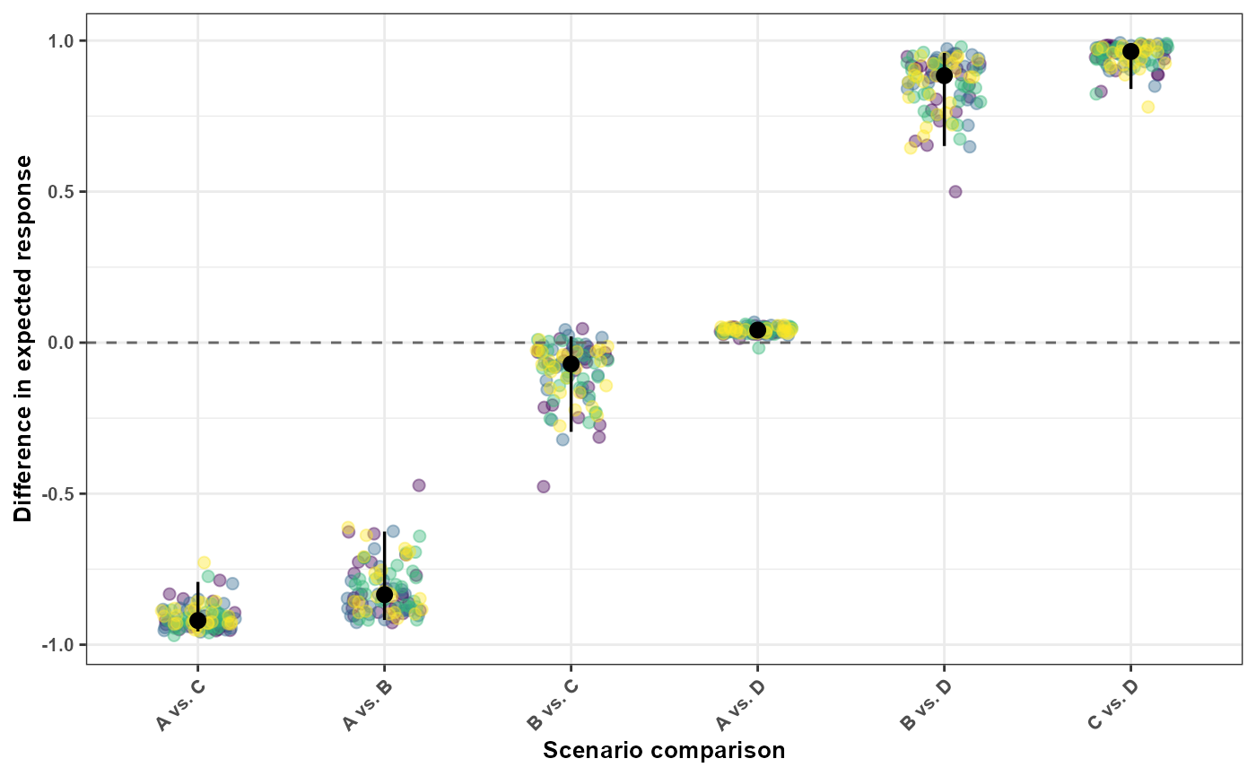

The colored points show the complete distribution of draw-specific differences for each scenario pair. The black point is the central difference reported in the summary output, while the vertical black line extends from diff_lower to diff_upper.

Values above zero indicate that the expected response for scenario2 is higher than the expected response for scenario1. Values below zero indicate that the expected response for scenario2 is lower. Comparisons whose uncertainty intervals cross zero include both positive and negative differences across the joint parameter draws.

These are joint environmental contrasts. Temperature, rainfall, and leaf wetness differ simultaneously among Scenarios A–D. The resulting differences therefore describe contrasts between complete multivariable environmental profiles and should not be interpreted as the isolated effect of any one exposure.

Comparing one exposure at a time

When the objective is to investigate a contrast involving one exposure, the remaining profiles should be held constant. The following example changes rainfall while maintaining the same temperature and leaf wetness profiles.

scenario_low_rain <- list(
  tmean = exposure_tmean_A,
  rain = simulate_exposures(
    max_lag = 85,
    mode = "profile",
    seed = 501,
    background = list(
      dist = "ar1",
      mean = 2,
      sd = 1,
      phi = 0.50
    ),
    n = 1
  ),
  wetness = exposure_wetness_A
)

scenario_high_rain <- list(
  tmean = exposure_tmean_A,
  rain = simulate_exposures(
    max_lag = 85,
    mode = "profile",
    seed = 502,
    background = list(
      dist = "ar1",
      mean = 15,
      sd = 3,
      phi = 0.50
    ),
    n = 1
  ),
  wetness = exposure_wetness_A
)

rainfall_comparison <- compare_predictions(
  fit = fit,
  profiles = list(
    low_rain = scenario_low_rain,
    high_rain = scenario_high_rain
  ),
  uncertainty = TRUE,
  output = "summary",
  n_samples = 100,
  seed = 123
)

rainfall_comparison
#>   scenario1 scenario2     pred1   pred1_sd pred1_lower pred1_upper     pred2
#> 1  low_rain high_rain 0.8852602 0.04879873   0.7618158   0.9553559 0.9981504
#>       pred2_sd pred2_lower pred2_upper      diff    diff_sd diff_lower
#> 1 0.0009853875   0.9952408   0.9991543 0.1133656 0.04937617 0.04094392
#>   diff_upper  abs_diff abs_diff_sd abs_diff_lower abs_diff_upper
#> 1  0.2372621 0.1133656  0.04937617     0.04094392      0.2372621
#>   percentage_point_change percentage_point_change_sd
#> 1                11.33656                   4.937617
#>   percentage_point_change_lower percentage_point_change_upper
#> 1                      4.094392                      23.72621
#>   relative_defined_fraction relative_change_defined    ratio   ratio_sd
#> 1                         1                    TRUE 1.128128 0.06699667
#>   ratio_lower ratio_upper percent_change percent_change_sd percent_change_lower
#> 1    1.042867    1.311432       12.81284          6.699667             4.286725
#>   percent_change_upper
#> 1             31.14316

Temperature and leaf wetness are identical in the two profiles. Therefore, the contrast is specifically associated with the change in the complete rainfall profile under the fitted multivariable model.

This remains a model-based associational comparison. It should not automatically be interpreted as the causal effect of intervening on rainfall unless the study design and assumptions support that interpretation.

Interpreting simulation and prediction outputs

Simulation and prediction tools provide related but distinct outputs:

simulate_exposures() creates one complete exposure profile;
simulate_ranges() constructs combinations of candidate exposure values;
simulate_scenarios() predicts outcomes over multiple scenarios;
predict_outcomes() predicts the expected response for complete profiles;
compare_exposures() compares the exposure profiles themselves;
compare_predictions() compares their model-based expected outcomes.

Before interpreting a result, verify:

whether the exposure profiles are chronological;
whether every profile contains max_lag + 1 observations;
whether all exposures required by the fitted model were supplied;
whether scenario values are supported by the observed data;
whether multiple exposures changed simultaneously;
whether uncertainty was propagated;
whether the output contains summaries or individual samples;
whether the prediction is population-level or group-specific;
whether the interpretation is associational or supported by a causal design.

Prediction is not observation simulation. predict_outcomes() returns the expected response under the fitted model. Parameter uncertainty can be propagated through coefficient draws, but this does not automatically add observation-level variability.

Summary

This section demonstrated how EpiExposure transforms a fitted DLNM into a framework for evaluating complete exposure profiles.

The workflow allows users to:

generate chronological exposure profiles;
add structured exposure patterns;
predict expected disease outcomes;
propagate parameter uncertainty;
evaluate scenario grids;
compare exposure profiles;
compare predicted responses.

These tools extend inference from the fitted exposure-lag surface to explicit, model-based comparisons of complete environmental profiles.

Next steps

The next section translates predicted disease outcomes into practical outcomes such as yield and economic losses using the simulate_losses() function.

These tools connect exposure-lag-response relationships with agronomic and economic consequences.

Ricardo G. Tomáz

Introduction

Preparing the example model

Complete exposure profiles

Simulating exposure profiles

Why simulate exposures?

Simulating a background process

Simulating structured exposure events

Predicting disease outcomes

Deterministic prediction

Prediction uncertainty

Scenario simulation

Why construct scenarios?

Defining epidemiological periods

Generating candidate scenarios

Predicting scenario outcomes

Summarizing scenario predictions

Visualizing summarized scenario predictions

Returning individual prediction samples

Visualizing individual prediction samples

Scenario surfaces

Comparing predictions

Comparing complete simulated profiles

Defining Scenario A

Defining Scenario B

Defining Scenario C

Defining Scenario D

Visualizing the candidate profiles

Comparing the exposure profiles

Comparing temperature profiles

Comparing rainfall profiles

Comparing leaf wetness profiles

Visualizing the exposure differences

Comparing the expected outcomes

Summarized comparisons

Draw-specific comparisons

Visualizing comparison uncertainty

Comparing one exposure at a time

Interpreting simulation and prediction outputs

Summary

Next steps