Get started with EpiExposure

What does `EpiExposure` do?

EpiExposure provides a standardized workflow for constructing, fitting, interpreting, and simulating distributed exposure-lag models in plant disease epidemiology.

The package helps users:

define non-linear exposure-lag structures;
fit distributed lag non-linear models;
quantify lag-specific, period-specific, and cumulative effects;
evaluate complete exposure profiles;
predict expected disease outcomes;
simulate alternative exposure scenarios;
estimate yield and economic losses.

Unlike conventional window-based approaches, EpiExposure treats the complete environmental profile preceding disease assessment as the epidemiological exposure unit.

What you will learn. This tutorial shows how to organize longitudinal epidemiological data, define and diagnose an exposure–lag structure, fit a first DLNM, and predict an expected disease outcome from a complete exposure profile.

The EpiExposure workflow

A basic analysis follows six stages:

organize and inspect complete exposure profiles;
define the exposure-response and lag-response basis functions;
evaluate the proposed structure for identifiability and numerical stability;
collapse each profile into one epidemic-level design row;
prepare the response and fit the model;
use the fitted model for interpretation, prediction, or simulation.

This section introduces the basic workflow but stops before detailed effect interpretation. Lag-specific, period-specific, and cumulative effects are covered in the Understanding Effects section

Organizing exposure profiles

EpiExposure expects longitudinal data in which each row represents one observation within an epidemic profile.

At minimum, the dataset must contain:

an epidemic identifier, such as epi_id;
a numeric temporal index, such as time;
one or more exposure variables;
one final response associated with each epidemic.

In the example dataset:

epi_id identifies independent epidemic profiles;
time orders observations chronologically;
tmean, rain, and wetness are environmental exposures;
y is the final disease response.

The temporal index begins at the earliest observation and ends at the disease assessment:

time 0  → earliest exposure observation → maximum lag
time 85 → disease assessment            → lag 0

Every epidemic must contain the same complete and regularly spaced exposure profile. With max_lag = 85, each epidemic requires:

$85 + 1 = 86$

observations for every fitted exposure.

library(EpiExposure)
library(ggplot2)

data("epi_data")

Inspecting the example dataset

The example contains complete environmental profiles for multiple epidemics.

epi_id	time	tmean	rain	wetness	y
1	0	21.96	0.00	8.83	0.33
1	1	21.47	0.00	11.86	0.33
1	2	21.53	5.38	12.49	0.33
1	3	21.76	14.59	12.30	0.33
1	4	20.83	0.00	11.41	0.33
1	5	23.03	8.24	7.98	0.33
1	6	23.89	4.69	10.84	0.33
1	7	23.14	12.30	8.58	0.33
1	8	25.32	4.14	10.61	0.33
1	9	25.99	1.91	14.10	0.33

Before modeling, verify that every epidemic contains the required number of observations:

table(
  table(
    epi_data$epi_id
  )
)
#> 
#>  86 
#> 520

For max_lag = 85, the expected result is 86 observations per epi_id.

Visualizing exposure profiles

Visual inspection can reveal temporal trends, unusual exposure profiles, limited variation, and missing observations.

wetness_plot = epi_data |>  
  ggplot(aes(time,wetness, group = epi_id))+
  geom_smooth(se = F, color = "#55A868",linewidth = 0.3)+
  theme_bw()+
  labs(x = "Days after planting the crop",
       y = "Leaf wetness (%)")+
  scale_x_continuous(limits = c(0,85), expand = c(0,0),
                     breaks = pretty(epi_data$time, n = 8))+
  theme(text = element_text(size = 10))


wetness_plot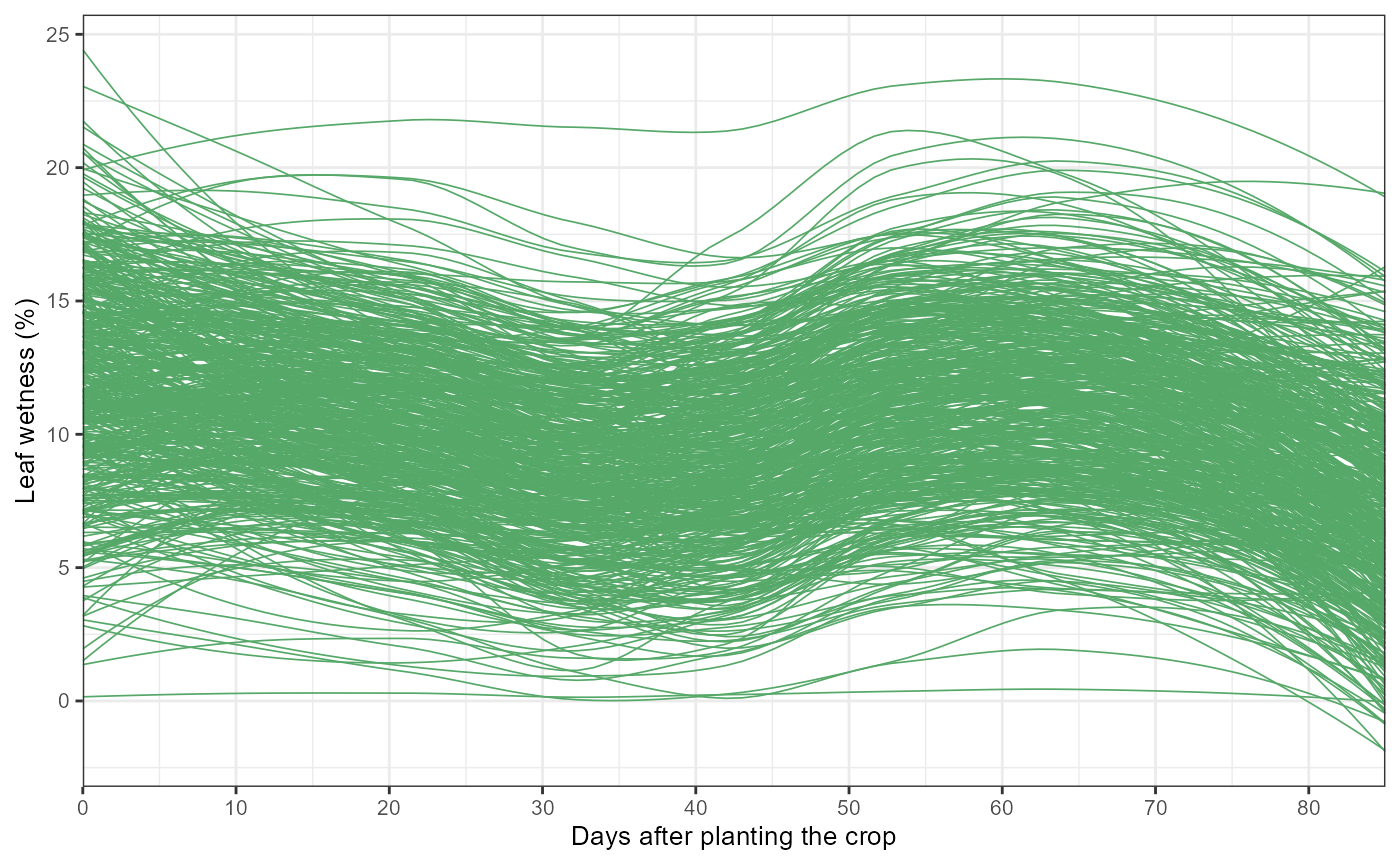

rain_plot = epi_data  |>  
  ggplot(aes(time,rain, group = epi_id))+
  geom_smooth(se = F, color = "#4C72B0",linewidth = 0.3)+
  theme_bw()+
  labs(x = "Days after planting the crop",
       y = "Daily precipitation (mm)")+
  scale_x_continuous(limits = c(0,85), expand = c(0,0),
                     breaks = pretty(epi_data$time, n = 8))+
  theme(text = element_text(size = 10))


rain_plot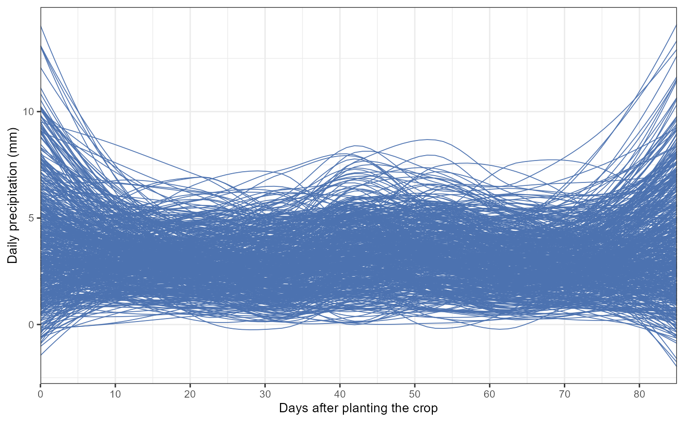

tmean_plot = epi_data |> 
  ggplot(aes(time,tmean, group = epi_id))+
  geom_smooth(se = F, color = "#C44E52",linewidth = 0.3)+
  theme_bw()+
  labs(x = "Days after planting the crop",
       y = "Mean temperature (°C)")+
  scale_x_continuous(limits = c(0,85), expand = c(0,0),
                     breaks = pretty(epi_data$time, n = 8))+
  theme(text = element_text(size = 10))


tmean_plot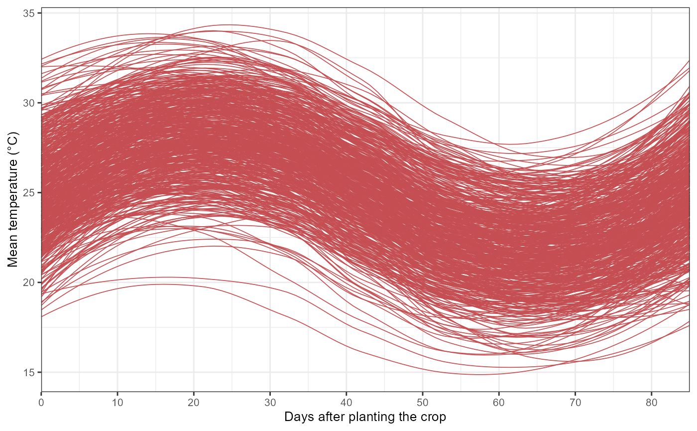

The objective is not to identify exposure effects visually. These plots only describe the observed profiles. Effect estimation requires the DLNM model.

Defining exposure-lag structures

The first modeling step is to define the non-linear exposure-response and lag-response basis functions.

cb <- define_exposures(
  data = epi_data,
  vars = c(
    "tmean",
    "rain",
    "wetness"
  ),
  max_lag = 85,
  df_var = 3,
  df_lag = 2
)

Here:

vars identifies the exposures included in the DLNM;
max_lag = 85 defines the retrospective lag window;
df_var = 3 controls exposure-response flexibility;
df_lag = 2 controls lag-response flexibility.

The resulting object stores the fitted basis definitions required for model construction and downstream prediction.

Exposure variables only. Coordinates, treatment groups, blocks, years, and other identifiers should not be included in vars. They can be preserved separately by build_design() when needed for random or spatial effects.

Checking identifiability and numerical stability

Before fitting the model, the proposed exposure–lag structure should be evaluated for identifiability and numerical stability. Increasing the number of exposures or the flexibility of the exposure and lag bases increases the number of cross-basis predictors and may produce redundant, rank-deficient, or poorly conditioned designs.

check_identifiability() reconstructs the same epidemic-level cross-basis design used by the EpiExposure fitting workflow. The function evaluates the combined numerical rank, scaled condition number, near-zero-variance columns, between-exposure cross-basis correlations, supplementary variance inflation factors, and the number of epidemics relative to design complexity.

identifiability <- check_identifiability(
  data = epi_data,
  vars = c(
    "tmean",
    "rain",
    "wetness"
  ),
  max_lag = 85,
  df_var = 3,
  df_lag = 2
)

The printed output classifies the proposed design as "ok", "warning", or "problem". The identifiable field indicates whether the combined epidemic-level design has full numerical rank, whereas numerically_stable additionally considers severe conditioning, near-zero-variance columns, and whether the available epidemics can support the number of design columns.

knitr::kable(
  utils::head(
    identifiability$overall,
    10L
  ),
  digits = 4,
  align = "c"
)

n_epidemics_total	n_epidemics_complete	n_epidemics_excluded	n_exposures	max_lag	history_length	crossbasis_columns	design_columns	rank	full_rank	rank_ratio	design_residual_df_proxy	condition_number_scaled	min_singular_value_scaled	max_singular_value_scaled	max_abs_crossbasis_correlation	median_abs_crossbasis_correlation	max_vif	median_vif	near_zero_variance_columns	epidemics_per_design_column	time_step
520	520	0	3	85	86	18	19	19	TRUE	1	501	18.8499	2.3269	43.8625	0.9177	0.0444	42.7938	5.2346	0	27.3684	1

knitr::kable(
  utils::head(
    identifiability$by_variable,
    10L
  ),
  digits = 4,
  align = "c"
)

variable	n_unique_exposure	history_length	max_lag	basis_columns	rank	full_rank	rank_ratio	condition_number_scaled	max_abs_within_basis_correlation
tmean	44611	86	85	6	6	TRUE	1	18.4765	0.8936
rain	15907	86	85	6	6	TRUE	1	7.2265	0.9177
wetness	44319	86	85	6	6	TRUE	1	4.7469	0.8108

knitr::kable(
  utils::head(
    identifiability$recommendations,
    10L
  ),
  digits = 4,
  align = "c"
)

x
6 cross-basis column(s) have VIF >= 10. Treat this as supplementary because spline-basis columns are correlated by construction. High VIF alone does not change `status`; prioritize the combined rank and scaled condition number.

A "warning" does not automatically invalidate the proposed structure. It indicates that the reported diagnostics should be examined before model fitting. A "problem" indicates rank deficiency or severe numerical instability and generally supports simplifying the candidate structure, for example by reducing df_var or df_lag, reconsidering redundant exposures, or increasing the number of independent epidemics.

The diagnostic thresholds are interpretive heuristics rather than universal inferential rules. In particular, high correlations or VIFs among individual spline columns may arise from the basis construction itself. The combined numerical rank and scaled condition number should therefore receive greater emphasis than any isolated column-level diagnostic.

Building the epidemic-level design

build_design() transforms each complete longitudinal profile into one epidemic-level row containing the cross-basis predictors.

dat <- build_design(
  data = epi_data,
  cb_templates = cb)

The original exposure columns are represented by canonical cross-basis columns such as:

cb_tmean_1, cb_tmean_2, ...
cb_rain_1, cb_rain_2, ...
cb_wetness_1, cb_wetness_2, ...

The coefficients of these columns should not be interpreted individually. Together, they reconstruct the non-linear exposure-lag-response association.

Inspect the resulting design:

First six rows of the epidemic-level DLNM design.
epi_id	cb_tmean_1	cb_tmean_2	cb_tmean_3	cb_tmean_4	cb_tmean_5	cb_tmean_6	cb_rain_1	cb_rain_2	cb_rain_3	cb_rain_4	cb_rain_5	cb_rain_6	cb_wetness_1	cb_wetness_2	cb_wetness_3	cb_wetness_4	cb_wetness_5	cb_wetness_6	y
1	5.765	5.545	21.801	0.515	-11.524	0.481	0.657	-0.839	16.376	2.138	-6.935	-1.236	4.869	0.929	23.264	1.555	-12.855	-0.774	0.330
2	5.838	7.070	20.565	0.978	-10.660	0.423	1.974	0.311	14.655	1.071	-4.947	0.128	-2.937	0.300	21.177	2.585	-12.003	-1.463	0.071
3	6.950	4.678	21.307	1.259	-10.660	0.061	1.180	0.384	5.205	0.195	-1.241	0.248	12.899	1.294	20.370	1.219	-8.147	0.539	0.190
4	7.156	8.038	20.828	0.221	-10.864	0.944	1.550	-0.018	7.855	-1.201	-2.977	0.685	-1.550	1.641	17.718	2.848	-9.977	-1.521	0.036
5	6.736	6.837	20.943	-0.178	-10.292	1.655	0.911	-0.435	7.176	-1.187	-2.442	0.382	1.169	-0.367	21.088	1.808	-11.570	-0.933	0.117
6	6.861	5.114	21.562	1.274	-11.556	-0.268	1.562	0.105	10.663	1.816	-3.284	-0.974	3.093	4.926	21.770	1.654	-11.816	-0.419	0.126

Preparing the disease response

The response must be prepared for the distribution used in the model.

dat <- prepare_response(
  data = dat,
  response = "y",
  family = "beta"
)

The Beta family is appropriate when the response is a continuous proportion strictly between 0 and 1.

Other supported families should be selected according to the response scale, for example:

binomial for a Bernoulli response coded as 0 or 1;
poisson for non-negative counts;
negative_binomial for overdispersed counts;
gamma for positive continuous responses;
gaussian for approximately continuous, unbounded responses.

For details on available modeling engines, supported response distributions, engine-specific requirements, and Bayesian and frequentist workflows, see the Advanced Topics section.

Fitting the first DLNM

The prepared design can now be fitted with one of the supported modeling engines.

fit <- fit_epidlnm(
  data = dat,
  model_engine = "glmmTMB",
  family = "beta",
  random_effect = NULL,
  epiexposure_spec = attr(
    cb,
    "spec"
  )
)

This model estimates a population-level association between the complete profiles of temperature, rainfall, and leaf wetness and the final disease response.

summary(fit)
#>  Family: beta  ( logit )
#> Formula:          
#> y_model ~ 1 + cb_tmean_1 + cb_tmean_2 + cb_tmean_3 + cb_tmean_4 +  
#>     cb_tmean_5 + cb_tmean_6 + cb_rain_1 + cb_rain_2 + cb_rain_3 +  
#>     cb_rain_4 + cb_rain_5 + cb_rain_6 + cb_wetness_1 + cb_wetness_2 +  
#>     cb_wetness_3 + cb_wetness_4 + cb_wetness_5 + cb_wetness_6
#> Data: dat
#> 
#>       AIC       BIC    logLik -2*log(L)  df.resid 
#>   -1375.4   -1290.4     707.7   -1415.4       500 
#> 
#> 
#> Dispersion parameter for beta family (): 29.7 
#> 
#> Conditional model:
#>               Estimate Std. Error z value Pr(>|z|)    
#> (Intercept)  -3.475218   0.947903  -3.666 0.000246 ***
#> cb_tmean_1    0.118230   0.014595   8.101 5.46e-16 ***
#> cb_tmean_2   -0.207029   0.027422  -7.550 4.36e-14 ***
#> cb_tmean_3   -0.062001   0.039492  -1.570 0.116421    
#> cb_tmean_4   -0.324065   0.100821  -3.214 0.001308 ** 
#> cb_tmean_5   -0.091731   0.031843  -2.881 0.003968 ** 
#> cb_tmean_6    0.016912   0.054302   0.311 0.755467    
#> cb_rain_1     0.217255   0.039357   5.520 3.39e-08 ***
#> cb_rain_2    -0.357518   0.050983  -7.013 2.34e-12 ***
#> cb_rain_3     0.239871   0.025436   9.431  < 2e-16 ***
#> cb_rain_4    -0.273807   0.039372  -6.954 3.54e-12 ***
#> cb_rain_5     0.160458   0.057216   2.804 0.005041 ** 
#> cb_rain_6    -0.034856   0.080037  -0.435 0.663201    
#> cb_wetness_1  0.110230   0.004315  25.545  < 2e-16 ***
#> cb_wetness_2 -0.037250   0.016298  -2.285 0.022284 *  
#> cb_wetness_3  0.074292   0.015282   4.861 1.17e-06 ***
#> cb_wetness_4 -0.039607   0.048578  -0.815 0.414877    
#> cb_wetness_5  0.090457   0.009308   9.718  < 2e-16 ***
#> cb_wetness_6 -0.055629   0.029369  -1.894 0.058207 .  
#> ---
#> Signif. codes:  0 '***' 0.001 '**' 0.01 '*' 0.05 '.' 0.1 ' ' 1

The individual cb_* coefficients are components of the cross-basis expansion. Their signs and $p$ -values should not be interpreted as isolated epidemiological effects.

The fitted exposure-lag surface must instead be reconstructed into quantities such as lag-specific, period-specific, and cumulative effects. That process is introduced in the Understanding Effects section

Predicting one complete exposure profile

A fitted model can also estimate the expected disease outcome associated with a complete hypothetical exposure profile.

In this example, a constant environmental scenario is evaluated over an 86-day exposure window. Daily mean temperature (tmean) is fixed at 25°C, daily rainfall (rain) at 5 mm, and daily leaf wetness duration (wetness) at 15 hours. The model combines the lagged contributions of all daily exposures to estimate the expected disease outcome for this exposure profile.

prediction <- predict_outcomes(
  fit = fit,
  profiles = list(
    tmean = rep(
      25,
      86
    ),
    rain = rep(
      5,
      86
    ),
    wetness = rep(
      15,
      86
    )
  )
)

prediction
#>   prediction
#> 1  0.9777891

Each exposure profile contains exactly 86 chronologically ordered observations, matching:

max_lag + 1

The resulting prediction represents the expected population-level disease response for the complete exposure profile. It is not a newly simulated observation.

Where to go next

You have now completed the basic EpiExposure workflow:

loaded longitudinal epidemic data;
inspected complete exposure profiles;
defined the exposure–lag basis;
evaluated its identifiability and numerical stability;
constructed the epidemic-level design;
prepared the response;
fitted a DLNM;
predicted an expected disease outcome.

Continue with the Understanding Effects section to learn how to:

interpret lag-specific effects;
define epidemiological periods;
calculate cumulative effects;
select meaningful reference exposures;
visualize uncertainty across the exposure-lag surface.

More advanced topics, including alternative modeling engines, random effects, spatial Matérn structures, and Bayesian estimation, are covered in the Advanced Topics section. Additional comparisons among candidate exposure–lag structures are discussed in the Sensitivity and Decision section.

Ricardo G. Tomáz

What does EpiExposure do?