Model Selection and Ensemble Forecasting

Ricardo G. Tomáz

Introduction

Distributed Lag Non-linear Models (DLNMs) require several modeling decisions, including:

• exposure variables;
• lag duration;
• exposure spline complexity;
• lag spline complexity;
• regression engine.

Different specifications may lead to different predictive performance.

EpiExposure provides tools for systematically exploring model configurations, ranking competing models, and combining predictions through ensemble forecasting.

This section demonstrates:

• automated DLNM model search;
• predictive validation;
• model ranking;
• ensemble forecasting;
• comparison of ensemble strategies.

Load example data

library(EpiExposure)
library(dplyr)
library(ggplot2)
library(patchwork)

data("epi_data")

head(epi_data, 10L )
#> # A tibble: 10 × 6
#>    epi_id  time tmean  rain wetness     y
#>     <dbl> <dbl> <dbl> <dbl>   <dbl> <dbl>
#>  1      1     0  22.0  0       8.83 0.330
#>  2      1     1  21.5  0      11.9  0.330
#>  3      1     2  21.5  5.38   12.5  0.330
#>  4      1     3  21.8 14.6    12.3  0.330
#>  5      1     4  20.8  0      11.4  0.330
#>  6      1     5  23.0  8.24    7.98 0.330
#>  7      1     6  23.9  4.69   10.8  0.330
#>  8      1     7  23.1 12.3     8.58 0.330
#>  9      1     8  25.3  4.14   10.6  0.330
#> 10      1     9  26.0  1.91   14.1  0.330

Why model selection matters

Exposure-lag-response relationships are highly sensitive to model specification.

For example, increasing lag flexibility may improve fit but increase overfitting.

Likewise, adding additional predictors may improve prediction in some pathosystems while reducing generalizability in others.

EpiExposure can evaluate predefined combinations of candidate DLNM specifications using a consistent fitting and validation workflow.

Searching candidate models

library(future)

future::plan(
  future::multisession,
  workers = 4
)

The appropriate number of workers depends on the available hardware and local computing policies. Users should avoid requesting more workers than their system can support.

future::plan(future::sequential ) 

Run the model search

best_models <- find_bestfit(
  data = epi_data,
  response = "y",
  group = "epi_id",
  time = "time",
  vars = c("tmean","rain","wetness"),
  max_lag = 85,
  df_var_grid = c(2,3,4),
  df_lag_grid = c(2,3,4),
  model_engine = "glmmTMB",
  family = "beta",
  keep_fits = TRUE)

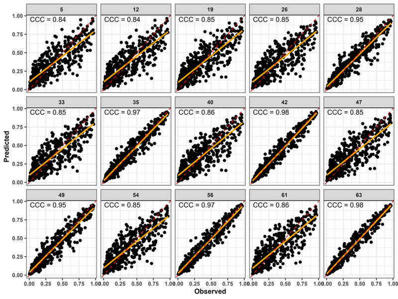
plot_performance(
  object = best_models,
  model_id = c(5,12,19,26,28,33,35,40,42,47,49,54,56,61,63),
  metrics = c("CCC"),
  x = "observed",
  y = "predicted",
  scale_factor = 1,
  ncol = 5,
  x_lab = "Observed ",
  y_lab = "Predicted",
  size = 1.4
) +
  ggplot2::theme(
    text = ggplot2::element_text(
      size = 10,
      face = "bold"
    )
  )

Observed versus predicted performance for selected candidate models

Inspect results

rank	model_id	df_var	df_lag	vars	n_vars	CCC	Cb	rho	RMSE	MAE	n_folds	n_success_folds	n_failed_folds	n_predictions	n_success	n_failed	n_warning_folds	warning_rate	n_warning_events	n_knot_warning_folds	n_convergence_warning_folds	n_hessian_warning_folds	n_other_warning_folds	n_knot_warning_events	n_convergence_warning_events	n_hessian_warning_events	n_other_warning_events
1	63	4	4	tmean + rain + wetness	3	0.9800	0.9997	0.9802	0.0529	0.0382	520	520	0	520	520	0	520	1	1010	520	490	0	0	520	490	0	0
2	42	3	4	tmean + rain + wetness	3	0.9783	0.9996	0.9786	0.0550	0.0395	520	520	0	520	520	0	520	1	523	520	3	0	0	520	3	0	0
3	56	4	3	tmean + rain + wetness	3	0.9702	0.9994	0.9708	0.0642	0.0475	520	520	0	520	520	0	520	1	530	520	10	0	0	520	10	0	0
4	35	3	3	tmean + rain + wetness	3	0.9688	0.9993	0.9695	0.0656	0.0483	520	520	0	520	520	0	520	1	520	520	0	0	0	520	0	0	0
5	49	4	2	tmean + rain + wetness	3	0.9523	0.9982	0.9540	0.0803	0.0577	520	520	0	520	520	0	520	1	520	520	0	0	0	520	0	0	0
6	28	3	2	tmean + rain + wetness	3	0.9493	0.9979	0.9513	0.0825	0.0589	520	520	0	520	520	0	520	1	520	520	0	0	0	520	0	0	0
7	40	3	4	tmean + wetness	2	0.8590	0.9863	0.8710	0.1316	0.0988	520	520	0	520	520	0	0	0	0	0	0	0	0	0	0	0	0
8	61	4	4	tmean + wetness	2	0.8575	0.9869	0.8689	0.1325	0.0998	520	520	0	520	520	0	0	0	0	0	0	0	0	0	0	0	0
9	19	2	4	tmean + wetness	2	0.8511	0.9834	0.8655	0.1343	0.1016	520	520	0	520	520	0	0	0	0	0	0	0	0	0	0	0	0
10	47	4	2	tmean + wetness	2	0.8482	0.9837	0.8623	0.1357	0.1035	520	520	0	520	520	0	0	0	0	0	0	0	0	0	0	0	0

Depending on the selected validation settings, the resulting object can include:

• a model identifier;
• the fitted predictor combination;
• exposure and lag spline settings;
• the modeling engine and response family;
• the Concordance Correlation Coefficient;
• the Root Mean Square Error;
• the Mean Absolute Error;
• bias-related metrics;
• the fitted model object when keep_fits = TRUE.

Ranking models

Top-performing models

The following example ranks models by decreasing CCC. This is one possible ranking criterion, not a universal rule. Candidate models should also be examined using error metrics, bias, convergence diagnostics, model complexity, and the scientific plausibility of the exposure-lag structure.

best_models %>%
  arrange(desc(CCC)) %>%
  select(
    model_id,
    vars,
    CCC,
    RMSE,
    MAE
  ) %>%
  head(10)
#> # A tibble: 10 × 5
#>    model_id vars                     CCC   RMSE    MAE
#>       <dbl> <chr>                  <dbl>  <dbl>  <dbl>
#>  1       63 tmean + rain + wetness 0.980 0.0529 0.0382
#>  2       42 tmean + rain + wetness 0.978 0.0550 0.0395
#>  3       56 tmean + rain + wetness 0.970 0.0642 0.0475
#>  4       35 tmean + rain + wetness 0.969 0.0656 0.0483
#>  5       49 tmean + rain + wetness 0.952 0.0803 0.0577
#>  6       28 tmean + rain + wetness 0.949 0.0825 0.0589
#>  7       40 tmean + wetness        0.859 0.132  0.0988
#>  8       61 tmean + wetness        0.858 0.132  0.0998
#>  9       19 tmean + wetness        0.851 0.134  0.102 
#> 10       47 tmean + wetness        0.848 0.136  0.104

Visualizing model performance

best_models %>%
  mutate(
    splines = paste(
      df_var,
      df_lag,
      sep = " × "
    )
  ) %>%
  ggplot(
    aes(
      Cb,
      CCC,
      color = splines
    )
  ) +
  geom_point(size = 3) +
  theme_bw()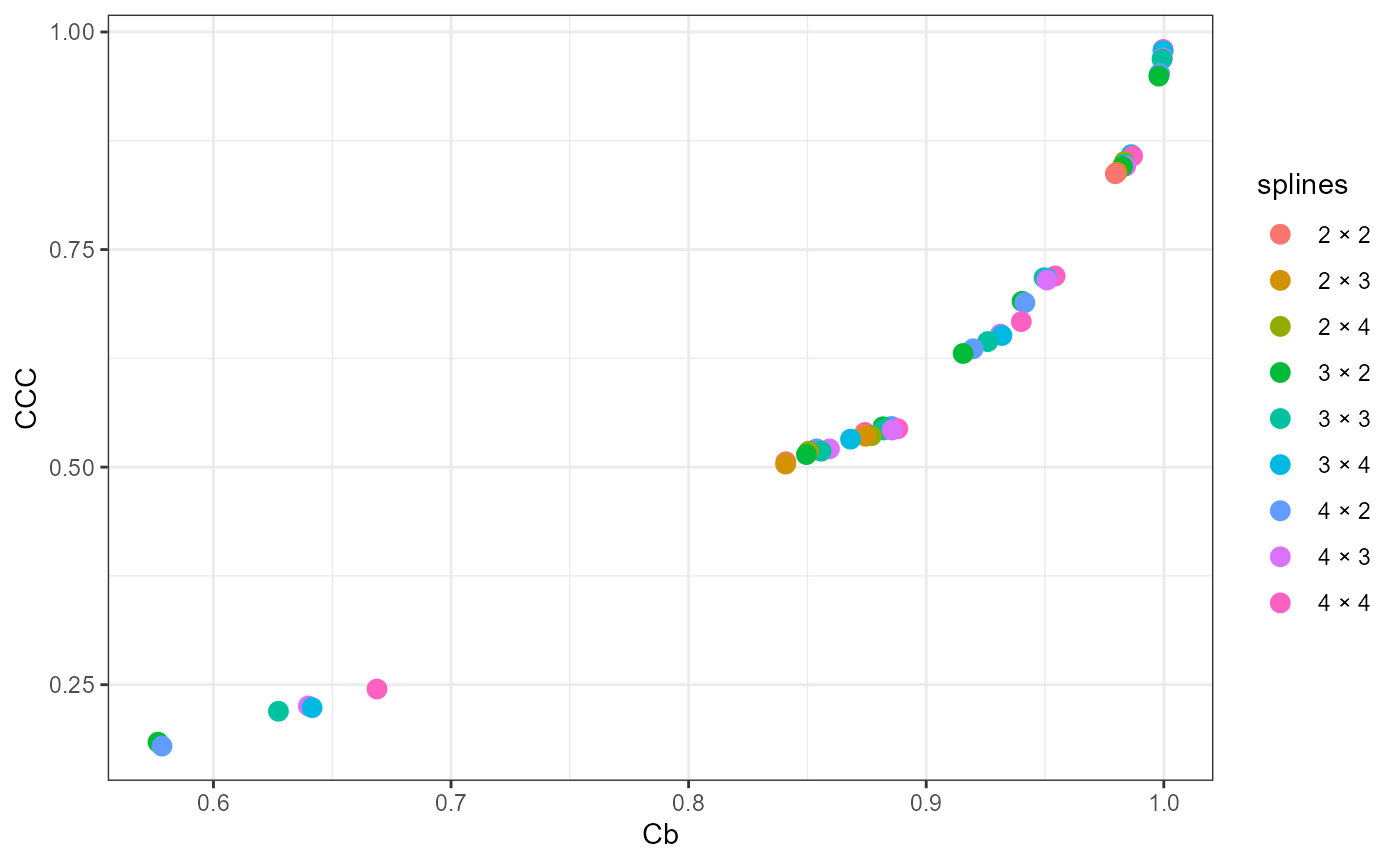

Understanding validation metrics

Concordance Correlation Coefficient

CCC evaluates agreement between observed and predicted outcomes by combining precision and accuracy.

Values closer to 1 indicate stronger concordance. However, CCC should be interpreted together with error and bias metrics rather than used as the only selection criterion.

Root Mean Square Error

RMSE summarizes the magnitude of prediction errors while assigning greater influence to larger errors because residuals are squared before averaging.

Lower values indicate better predictive performance when models are evaluated on the same response scale and validation data.

Mean Absolute Error

MAE is the average absolute difference between observed and predicted outcomes.

Lower values indicate better predictive performance. Because MAE remains on the response scale, it is often easier to interpret directly than RMSE.

Inspecting specific models

Suppose the best model is:

top_model <- best_models |>
  dplyr::arrange(
    dplyr::desc(
      CCC
    )
  ) |>
  dplyr::slice(
    1L
  )

Why use ensembles?

No single model is guaranteed to be optimal.

Different DLNM structures frequently capture different aspects of the underlying epidemiological process.

Combining predictions from multiple models often improves stability and predictive robustness.

Selecting ensemble candidates

The identifiers below are illustrative. Replace them with model identifiers selected from the user’s own best_models object.

candidate_models <- c(
  63,
  23,
  44
)

Therefore, three candidate models (best ranked [63], and the two lower-ranked models [23, 44]) were selected to be used on the ensemble approaches, with CCC used as the performance metric for the weighted ensemble.

Unweighted ensemble

ens_unweighted <- ensemble_bestfit(
  bestfit = best_models,

  ensemble_scope = "model",

  method = "unweighted",

  model_id = candidate_models)

Inspect results

The ensemble summary can be extracted from the fitted ensemble object:

ens_unweighted$ensemble_summary

method	n_models	n_oof	family	outcome_type	cv_method	cv_scheme	k	weight_metric	metric_direction	threshold	stacking_model	stack_objective	stack_intercept	weight_transform	CCC	Cb	rho	RMSE	MAE
unweighted	3	520	beta	non_binary	LOOCV	leave_one_group_out	520	CCC	maximize	NA	NA	NA	NA	NA	0.6455	0.739	0.8735	0.1741	0.1476

Weighted ensemble

ens_weighted <- ensemble_bestfit(
  bestfit = best_models,

  ensemble_scope = "model",

  method = "weighted",

  model_id = candidate_models,

  weight_metric = "CCC",

  weight_transform = "rank_inverse"
)

Inspect results

The ensemble summary can be extracted from the fitted ensemble object:

ens_weighted$ensemble_summary

method	n_models	n_oof	family	outcome_type	cv_method	cv_scheme	k	weight_metric	metric_direction	threshold	stacking_model	stack_objective	stack_intercept	weight_transform	CCC	Cb	rho	RMSE	MAE
weighted	3	520	beta	non_binary	LOOCV	leave_one_group_out	520	CCC	maximize	NA	NA	NA	NA	rank_inverse	0.8386	0.8788	0.9542	0.125	0.1053

Stacked ensemble

ens_stacked <- ensemble_bestfit(
  bestfit = best_models,

  ensemble_scope = "model",

  method = "stacked",

  model_id = candidate_models,

  stacking_model = "ridge",

  stack_objective = "regularized"
)

Inspect results

The ensemble summary can be extracted from the fitted ensemble object:

ens_stacked$ensemble_summary

method	n_models	n_oof	family	outcome_type	cv_method	cv_scheme	k	weight_metric	metric_direction	threshold	stacking_model	stack_objective	stack_intercept	weight_transform	CCC	Cb	rho	RMSE	MAE
stacked	3	520	beta	non_binary	LOOCV	leave_one_group_out	520	CCC	maximize	NA	ridge	regularized	-0.004	NA	0.9798	0.9998	0.98	0.0532	0.0385

Comparing ensemble strategies

ensemble_metrics <- dplyr::bind_rows(
  Unweighted = ens_unweighted$ensemble_summary,
  Weighted = ens_weighted$ensemble_summary,
  Stacked = ens_stacked$ensemble_summary,
  .id = "method"
) |>
  dplyr::select(
    method,
    CCC,
    RMSE,
    MAE
  )

ensemble_metrics
#> # A tibble: 3 × 4
#>   method       CCC   RMSE    MAE
#>   <chr>      <dbl>  <dbl>  <dbl>
#> 1 Unweighted 0.646 0.174  0.148 
#> 2 Weighted   0.839 0.125  0.105 
#> 3 Stacked    0.980 0.0532 0.0385

Visualizing ensemble predictions

ens_unweighted$ensemble_predictions$method = "unweighted"
ens_weighted$ensemble_predictions$method = "weighted"
ens_stacked$ensemble_predictions$method = "stacked"

ensemble_all = rbind(ens_unweighted$ensemble_predictions,ens_weighted$ensemble_predictions, ens_stacked$ensemble_predictions)

knitr::kable(utils::head(ensemble_all, 10L),
              digits = 4, align = "c" )

group	fold	method	observed	predicted_ensemble	model_63	model_23	model_44
1	1	unweighted	0.3299	0.4712	0.3653	0.5205	0.5277
2	2	unweighted	0.0706	0.3607	0.0776	0.4947	0.5098
3	3	unweighted	0.1900	0.2310	0.1939	0.2508	0.2483
4	4	unweighted	0.0356	0.2738	0.0477	0.3806	0.3931
5	5	unweighted	0.1173	0.2811	0.1206	0.3630	0.3597
6	6	unweighted	0.1262	0.3007	0.1403	0.3811	0.3808
7	7	unweighted	0.2764	0.2737	0.2366	0.2919	0.2926
8	8	unweighted	0.3777	0.3836	0.4355	0.3595	0.3559
9	9	unweighted	0.0250	0.1886	0.0228	0.2711	0.2718
10	10	unweighted	0.8908	0.5461	0.9030	0.3732	0.3620

ensemble_metrics$method = c("unweighted","weighted","stacked")

ordem_methods <- c(
  "unweighted",
  "weighted",
  "stacked"
)

ensemble_plot <- ensemble_all %>%
  filter(!is.na(method)) %>%
  mutate(
    method = as.character(method)
  ) %>%
  filter(method %in% ordem_methods) %>%
  mutate(
    method = factor(
      method,
      levels = ordem_methods
    )
  )



CCC_plot <- ensemble_metrics %>%
  mutate(
    method = factor(
      method,
      levels = ordem_methods
    )
  )



pos_CCC <- ensemble_plot %>%
  group_by(method) %>%
  summarise(
    x = min(observed, na.rm = TRUE) +
      0.05 * diff(range(observed, na.rm = TRUE)),
   
    y = max(predicted_ensemble, na.rm = TRUE) -
      0.05 * diff(range(predicted_ensemble, na.rm = TRUE)),
   
    .groups = "drop"
  ) %>%
  left_join(
    CCC_plot %>% select(method, CCC),
    by = "method"
  )



 ensemble_gg = ggplot(ensemble_plot,
            aes(observed, predicted_ensemble)) +
  geom_point()+
  geom_smooth(method = "lm",se = FALSE, color = "orange") +
  geom_abline(
    intercept = 0,
    slope = 1,
    color = "red",
    linetype = "dashed",
    linewidth = 1) +
  geom_text(
    data = pos_CCC,
    aes(
      x = 0.02,
      y = 0.97,
      label = sprintf("CCC = %.2f", CCC)
    ),
    inherit.aes = FALSE,
    hjust = 0,
    vjust = 1,
    size = 4) +
  facet_wrap(
    ~method,
    ncol = 1) +
  theme_bw() +
    scale_x_continuous(
    limits = c(0, 1),
    breaks = seq(0, 1, 0.20),
    expand = expansion(mult = 0.03)
  ) +
 
  scale_y_continuous(
    limits = c(0, 1),
    breaks = seq(0, 1, 0.20),
    expand = expansion(mult = 0.03)
  ) +
  labs(
    x = "Observed",
    y = "Predicted") +
  theme(text = element_text(size = 10,face = "bold"),legend.position = "none")
 
 ensemble_gg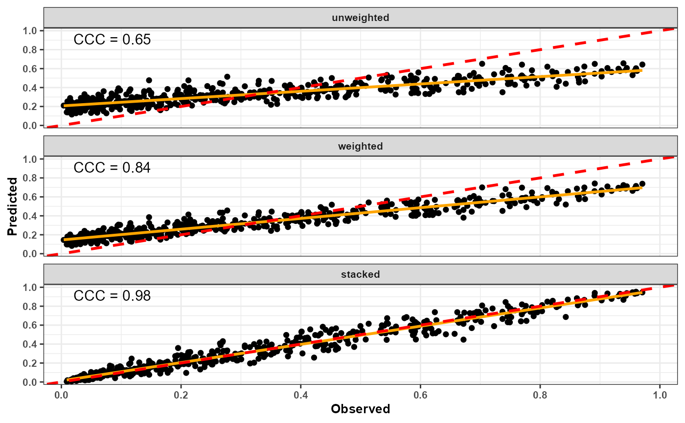

best_models_plot <- best_models %>%
   mutate(
    splines = paste(df_lag, df_var, sep = " x ")
  )


best_plot <- best_models_plot %>%
  ggplot(aes(
    Cb, CCC,
    color = as.factor(splines),
    shape = as.factor(vars)
  )) +
 
  geom_point(size = 4) +
 
  scale_color_viridis_d() +
 
  labs(
    x = "Cb",
    y = "CCC",
    color = "Splines",
    shape = "Predictors"
  ) +
 
  guides(
    color = guide_legend(
      position = "top",
      nrow = 1,
      byrow = TRUE,
      title.position = "left",
      theme = theme(
        legend.key.height = unit(0.25, "cm"),
        legend.key.width = unit(0.45, "cm"),
        legend.spacing.y = unit(0, "cm"),
        legend.margin = margin(
          t = -3,
          r = 0,
          b = -3,
          l = 0
        )
      )
    ),
   
    shape = guide_legend(
      position = "right"
    )
  ) +
 
  theme_bw() +
 
  theme(
    text = element_text(
      size = 10,
      face = "bold"
    )
  )

final_plot <- ensemble_gg + best_plot +
  plot_layout(ncol = 2) +
  plot_annotation(
    tag_levels = "a",
    tag_prefix = "(",
    tag_suffix = ")"
  ) &
  theme(
    plot.tag = element_text(
      size = 12,
      face = "bold"
    ),
    plot.tag.position = c(0.02, 0.94)
  )

final_plot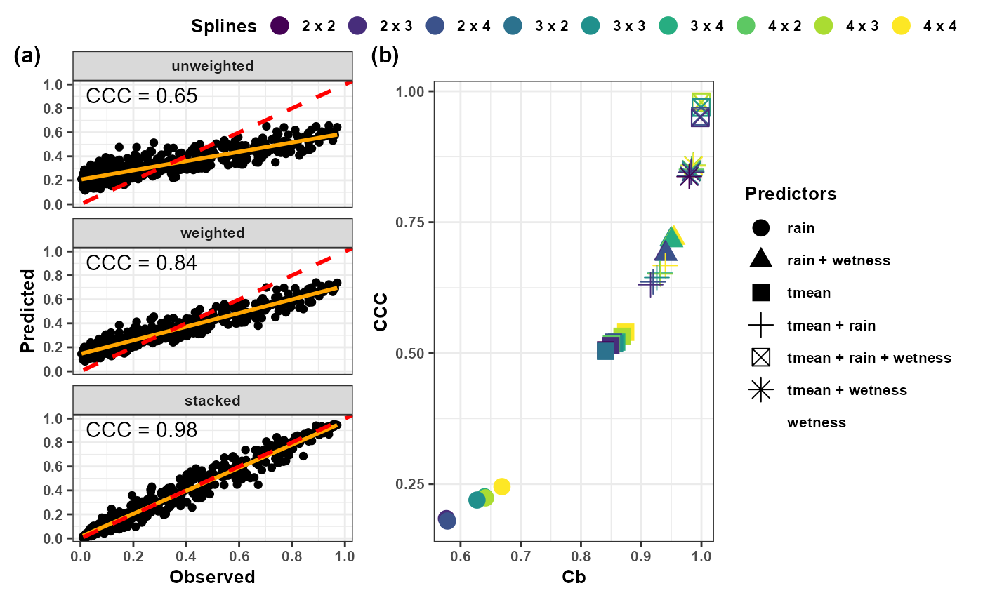

Choosing a model-level ensemble strategy

Each ensemble method has advantages.

Unweighted ensemble

• gives equal contribution to the selected models;
• is simple and transparent;
• avoids estimating additional model weights;
• can be affected by weak or redundant candidate models.

Weighted ensemble

• assigns different contributions to candidate models;
• can emphasize models with stronger validation performance;
• depends on the selected metric and weight transformation;
• does not guarantee improvement over the best individual model.

Stacked ensemble

• estimates combination coefficients from model predictions;
• can account for complementary predictive information;
• requires careful separation between weight estimation and final evaluation;
• can overfit when the validation sample is limited or when candidate predictions are highly similar.

Therefore, no ensemble method is universally superior.

An unweighted ensemble is useful as a transparent reference because every candidate contributes equally.

A weighted ensemble is appropriate when the selected validation metric provides a defensible basis for assigning model contributions.

A stacked ensemble can be useful when candidate models contain complementary predictive information and the stacking weights are estimated without using the same observations reserved for final evaluation.

Regardless of the method, compare the ensemble against:

• the strongest individual candidate;
• a simple baseline model;
• alternative ensemble strategies;
• results on validation data not reused for weight estimation.

The previous sections focused on model-level ensembles, which combine out-of-fold predictions and evaluate their predictive performance.

EpiExposure can also construct lag-contribution ensembles. Instead of combining predicted outcomes, these ensembles combine the lag-specific ECI decompositions obtained from selected full-data model refits.

Lag-contribution ensembles

Why construct a lag ensemble?

Model-level ensembles combine predictions from multiple candidate models. However, models may also differ in how they distribute the contribution of an exposure across the fitted lag interval.

A lag ensemble combines the lag-specific epidemiological contribution indices obtained from the selected models. For lag $l$, the ensemble contribution is defined as:

$$ECI_{\mathrm{ensemble},l} = \sum_m \alpha_m ECI_{m,l},$$

where $ECI_{m,l}$ is the lag-specific weighted ECI from model $m$, and $\alpha_m$ is the model weight derived from out-of-fold model performance.

The model weights therefore come from cross-validation, whereas the lag-specific ECI values are calculated from the selected models refitted to the complete dataset.

Lag ensembles require retained full-data fits or precomputed lag data. For automatic lag decomposition, best_models must be the complete object returned by find_bestfit() and must contain the retained fitted models in attr(best_models, "fits"). An Excel or CSV export of the ranking table does not preserve the attributes, fitted models, or basis metadata required for this calculation.

The fitted models are not used to recalculate the cross-validation metrics. The model ranking and ensemble weights remain based on the out-of-fold predictions produced by find_bestfit(). The retained full-data fits are used only to obtain the final lag-specific decompositions for the selected models.

Constructing unweighted and weighted lag ensembles

The following example selects the three highest-ranked models and constructs two lag ensembles:

• "unweighted" gives equal weight to each selected model;
• "weighted" derives model weights from the selected performance metric.

To keep the example computationally efficient, the lag ensemble is demonstrated using one complete epidemic profile. Users may instead supply all available epidemic profiles, provided that each profile contains the complete max_lag + 1 observations required by the fitted models. The computational cost will increase with the number of epidemics, exposures, selected models, and lags. The results shown here are therefore specific to Epidemic 1.

epi_data1 = epi_data |> 
  filter(epi_id == 1)

lag_ensemble <- ensemble_bestfit(
  bestfit = best_models,
  data = epi_data1,
  group = "epi_id",
  var = c(
    "tmean",
    "rain",
    "wetness"
  ),
  ensemble_scope = "lag",
  method = c(
    "unweighted",
    "weighted"
  ),
  top_n = 3,
  weight_metric = NULL,
  weight_transform = "softmax",
  lag_group_cols = c(
    "epi_id",
    "var",
    "lag"
  ),
  lg_strategy = "requested_available",
  rl_weights = TRUE,
  compute_ecilag_args = list(
    uncertainty = FALSE
  ),
  verbose = TRUE
)

When weight_metric = NULL, ensemble_bestfit() uses the ranking metric stored by find_bestfit(). The direction of that metric is handled automatically: metrics such as CCC are maximized, whereas metrics such as RMSE are minimized.

The argument:

lg_strategy = "requested_available"

uses each requested exposure when that exposure is available in the selected model. Because candidate models may contain different combinations of exposures, not every model necessarily contributes to every exposure-specific lag ensemble.

With:

rl_weights = TRUE

the model weights are renormalized among the models available for each exposure-lag unit. This ensures that the available model weights sum to one within each lag-specific ensemble calculation.

Inspecting selected models and weights

The selected candidate models can be inspected directly:

lag_ensemble$selected_models

rank	model_id	df_var	df_lag	vars	n_vars	CCC	Cb	rho	RMSE	MAE	n_folds	n_success_folds	n_failed_folds	n_predictions	n_success	n_failed	n_warning_folds	warning_rate	n_warning_events	n_knot_warning_folds	n_convergence_warning_folds	n_hessian_warning_folds	n_other_warning_folds	n_knot_warning_events	n_convergence_warning_events	n_hessian_warning_events	n_other_warning_events
1	63	4	4	tmean + rain + wetness	3	0.9800	0.9997	0.9802	0.0529	0.0382	520	520	0	520	520	0	520	1	1010	520	490	0	0	520	490	0	0
2	42	3	4	tmean + rain + wetness	3	0.9783	0.9996	0.9786	0.0550	0.0395	520	520	0	520	520	0	520	1	523	520	3	0	0	520	3	0	0
3	56	4	3	tmean + rain + wetness	3	0.9702	0.9994	0.9708	0.0642	0.0475	520	520	0	520	520	0	520	1	530	520	10	0	0	520	10	0	0

The model weights used by each ensemble method are stored separately:

lag_ensemble$model_weights

method	model_id	metric_value	prediction_weight	lag_weight
unweighted	63	0.9800	NA	0.3333
unweighted	42	0.9783	NA	0.3333
unweighted	56	0.9702	NA	0.3333
weighted	63	0.9800	NA	0.3346
weighted	42	0.9783	NA	0.3340
weighted	56	0.9702	NA	0.3314

For the unweighted ensemble, the selected models receive equal lag weights. For the weighted ensemble, the weights are derived from the selected cross-validation performance metric.

These weights describe the relative influence of the selected models in the lag ensemble. They are not lag-specific DLNM coefficients.

Inspecting ensemble lag contributions

The combined lag-specific contributions are returned in:

lag_ensemble$ensemble_by_lag

Inspect the first rows:

epi_id	var	lag	method	ECI_weighted_ens	n_models	n_selected_models	raw_model_weight_sum	weights_renormalized	models_used	ECI_percent_ens
1	tmean	0	unweighted	-0.0189	3	3	1	TRUE	42, 56, 63	1.4481
1	tmean	1	unweighted	-0.0167	3	3	1	TRUE	42, 56, 63	1.2743
1	tmean	2	unweighted	-0.0242	3	3	1	TRUE	42, 56, 63	1.8470
1	tmean	3	unweighted	-0.0181	3	3	1	TRUE	42, 56, 63	1.3854
1	tmean	4	unweighted	-0.0180	3	3	1	TRUE	42, 56, 63	1.3787
1	tmean	5	unweighted	-0.0182	3	3	1	TRUE	42, 56, 63	1.3889
1	tmean	6	unweighted	-0.0268	3	3	1	TRUE	42, 56, 63	2.0472
1	tmean	7	unweighted	-0.0180	3	3	1	TRUE	42, 56, 63	1.3757
1	tmean	8	unweighted	0.0090	3	3	1	TRUE	42, 56, 63	0.6871
1	tmean	9	unweighted	0.0268	3	3	1	TRUE	42, 56, 63	2.0466
1	tmean	10	unweighted	0.0129	3	3	1	TRUE	42, 56, 63	0.9838
1	tmean	11	unweighted	-0.0279	3	3	1	TRUE	42, 56, 63	2.1334

The principal output columns are:

• var: exposure variable;
• lag: retrospective lag, where lag 0 is the most recent exposure;
• method: ensemble method;
• ECI_weighted_ens: signed ensemble ECI contribution at that lag;
• ECI_percent_ens: absolute percentage contribution of that lag within the corresponding exposure and ensemble method;
• n_models: number of models contributing to that lag unit;
• raw_model_weight_sum: total original model-weight mass available for that lag unit;
• weights_renormalized: whether weights were renormalized among the available models;
• models_used: selected models contributing to the lag unit.

The signed value ECI_weighted_ens preserves the direction of the ensemble contribution. In contrast, ECI_percent_ens is based on the absolute contribution magnitude and describes how the total lag contribution is distributed across the fitted lag interval.

Visualizing signed lag contributions

ensemble_by_lag = lag_ensemble$ensemble_by_lag

lag_ensemble_signed_plot <- ggplot(
  ensemble_by_lag,
  aes(
    x = lag,
    y = ECI_weighted_ens,
    color = method
  )
) +
  geom_hline(
    yintercept = 0,
    color = "grey50",
    linetype = "dashed",
    linewidth = 0.5
  ) +
  geom_line(
    linewidth = 1
  ) +
  facet_wrap(
    vars(var),
    ncol = 1,
    scales = "free_y",
    labeller = as_labeller(
      c(
        tmean = "Mean temperature",
        rain = "Rainfall",
        wetness = "Leaf wetness"
      )
    )
  ) +
  scale_x_reverse(
    breaks = seq(
      0,
      85,
      by = 15
    )
  ) +
  scale_color_manual(
    values = c(
      unweighted = "#4C72B0",
      weighted = "#C44E52"
    ),
    labels = c(
      unweighted = "Unweighted",
      weighted = "Weighted"
    )
  ) +
  theme_bw() +
  labs(
    x = "Retrospective lag",
    y = "Ensemble weighted ECI",
    color = "Ensemble method"
  ) +
  theme(
    text = element_text(
      size = 10,
      face = "bold"
    ),
    strip.background = element_rect(
      fill = "white",
      color = "black"
    ),
    strip.text = element_text(
      face = "bold"
    ),
    legend.position = "top"
  )

lag_ensemble_signed_plot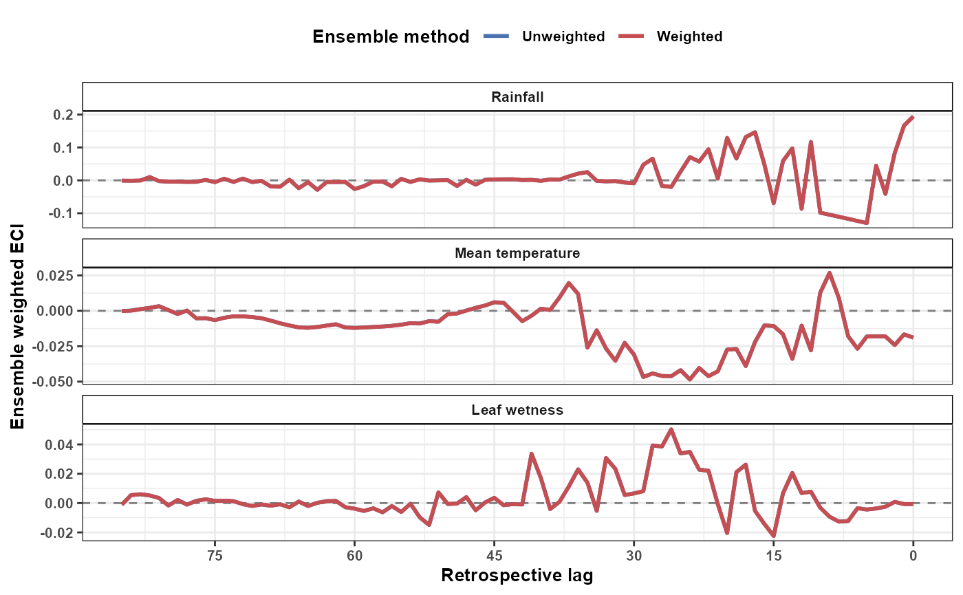

The lag axis is displayed retrospectively. Lag 0 corresponds to the most recent exposure observation, whereas increasing lag values represent progressively older exposure conditions.

Positive and negative values describe the direction of the combined lag-specific contribution. The weighted and unweighted curves may differ when the selected models receive substantially different performance-based weights.

Visualizing relative lag contributions

The percentage contribution provides a complementary interpretation based on the absolute contribution magnitude:

lag_ensemble_percent_plot <- ggplot(
  ensemble_by_lag,
  aes(
    x = lag,
    y = ECI_percent_ens,
    color = method
  )
) +
  geom_line(
    linewidth = 1
  ) +
  facet_wrap(
    vars(var),
    ncol = 1,
    scales = "free_y",
    labeller = as_labeller(
      c(
        tmean = "Mean temperature",
        rain = "Rainfall",
        wetness = "Leaf wetness"
      )
    )
  ) +
  scale_x_reverse(
    breaks = seq(
      0,
      85,
      by = 15
    )
  ) +
  scale_color_manual(
    values = c(
      unweighted = "#4C72B0",
      weighted = "#C44E52"
    ),
    labels = c(
      unweighted = "Unweighted",
      weighted = "Weighted"
    )
  ) +
  theme_bw() +
  labs(
    x = "Retrospective lag",
    y = "Absolute lag contribution (%)",
    color = "Ensemble method"
  ) +
  theme(
    text = element_text(
      size = 10,
      face = "bold"
    ),
    strip.background = element_rect(
      fill = "white",
      color = "black"
    ),
    strip.text = element_text(
      face = "bold"
    ),
    legend.position = "top"
  )

lag_ensemble_percent_plot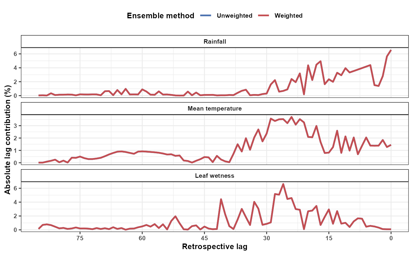

ECI_percent_ens is calculated from the absolute lag contributions within each exposure and ensemble method. Consequently, the percentages describe where the ensemble contribution is concentrated across lags, but they do not preserve the positive or negative direction of that contribution.

The signed and percentage plots should therefore be interpreted together:

• ECI_weighted_ens describes the direction and magnitude of the combined contribution;
• ECI_percent_ens describes the relative concentration of absolute contribution across lags.

Using strict exposure availability

The previous example used:

lg_strategy = "requested_available"

which allows different selected models to contribute to different exposures when their fitted variable sets differ.

For a stricter comparison, the user can require every selected model to contain all requested exposures:

lag_ensemble_strict <- ensemble_bestfit(
  bestfit = best_models,
  data = epi_data1,
  group = "epi_id",
  var = c(
    "tmean",
    "rain",
    "wetness"
  ),
  ensemble_scope = "lag",
  method = c(
    "unweighted",
    "weighted"
  ),
  top_n = 3,
  weight_transform = "softmax",
  lag_group_cols = c(
    "epi_id",
    "var",
    "lag"
  ),
  lg_strategy = "strict",
  rl_weights = TRUE,
  compute_ecilag_args = list(
    uncertainty = FALSE
  )
)

This strict mode stops when a selected model does not contain one of the requested exposures or when a lag unit is not available from every selected model. It is useful when the analyst wants the same model set to support every exposure-specific lag ensemble.

Lag-ensemble uncertainty is not generated in EpiExposure v1. The selected models are fitted separately, and independently sampled coefficient or posterior draws do not define a valid joint draw distribution across models. For this reason, ensemble_bestfit() combines deterministic lag-specific ECI decompositions and does not pair arbitrary draw indices across fitted models.

Lag ensembles should be interpreted as model-performance-weighted summaries of lag-specific ECI contributions. They do not replace external validation, do not represent raw DLNM coefficients, and should not be interpreted as causal attribution across lags.

Avoiding optimistic ensemble evaluation

Ensemble weights should be estimated from out-of-sample or cross-validated predictions whenever possible. Estimating weights and reporting performance on the same fitted predictions can produce optimistic results.

The final evaluation should use observations that were not reused to select candidate models or estimate ensemble weights. If a completely independent test set is unavailable, nested or repeated cross-validation may provide a more defensible assessment.

Summary

This section introduced the EpiExposure model-selection and ensemble framework.

The workflow includes:

• defining a candidate model space;
• fitting candidate DLNM specifications;
• evaluating predictive performance;
• ranking models using multiple criteria;
• retaining selected fitted models;
• combining predictions through unweighted, weighted, or stacked ensembles;
• comparing ensemble predictions with individual models and simple baselines.

Model selection and ensemble construction do not remove model uncertainty. Their value depends on the candidate model space, validation design, selection rules, and independence of the final performance assessment.