Sensitivity Analysis and Decision Support

Ricardo G. Tomáz

Introduction

Exposure-response relationships are often non-linear. A small change in an environmental exposure may correspond to little change in the expected disease response in one region of the fitted curve but a much larger change in another.

Effect summaries describe the direction and magnitude of modeled associations. Sensitivity analysis addresses a complementary question:

Where does the model-predicted disease response change most rapidly as an exposure changes?

EpiExposure provides tools for examining:

• local rates of change along prediction curves;
• proportional response changes through elasticity;
• model-derived critical exposure regions;
• differences in sensitivity among environmental drivers;
• potential regions of interest for monitoring and decision support.

What you will learn. This tutorial shows how to generate controlled exposure gradients, predict disease responses along those gradients, calculate local sensitivity and elasticity, and identify regions in which the fitted response changes most rapidly.

Sensitivity results describe mathematical features of the fitted model. They do not automatically establish biological thresholds, causal intervention points, or management recommendations. Such interpretations require biological validation and decision criteria appropriate to the pathosystem.

Preparing the example model

This section uses the same example dataset and DLNM specification introduced in the previous tutorials.

library(EpiExposure)
library(dplyr)
library(ggplot2)

data(
  "epi_data")

Define the exposure-lag structures:

cb <- define_exposures(
  data = epi_data,
  vars = c(
    "tmean",
    "rain",
    "wetness"
  ),
  max_lag = 85,
  df_var = 3,
  df_lag = 2
)

Build the epidemic-level design:

dat <- build_design(
  data = epi_data,
  cb_templates = cb
)

Prepare the disease response:

dat <- prepare_response(
  data = dat,
  response = "y",
  family = "beta"
)

Fit the DLNM:

fit <- fit_epidlnm(
  data = dat,
  model_engine = "glmmTMB",
  family = "beta",
  random_effect = NULL,
  epiexposure_spec = attr(
    cb,
    "spec"
  )
)

The fitted model is now used to predict the expected disease response along controlled environmental gradients.

From effect interpretation to sensitivity analysis

The Understanding Effects section introduced lag-specific, period-specific, and cumulative summaries of the fitted exposure-lag-response relationship.

Sensitivity analysis provides a different view. Rather than summarizing the magnitude of an effect at an exposure-lag combination, it estimates how rapidly the predicted response changes along a selected exposure gradient.

Conceptually:

effect analysis
    → What modeled contrast is associated with an exposure?

sensitivity analysis
    → How rapidly does the predicted response change as the exposure changes?

The two approaches are complementary. A region can have a relatively large predicted response but low sensitivity if the curve is locally flat. A region with a moderate predicted response can have high sensitivity if the curve is changing rapidly.

Generating controlled exposure gradients

The sensitivity workflow uses simulate_ranges() and simulate_scenarios() to create controlled exposure gradients.

In this section, these functions are used specifically to evaluate one environmental variable across a sequence of values while the remaining variables are held constant.

The broader use of simulation tools for constructing complete exposure profiles, structured events, and multivariable scenarios is covered in the Simulation and Prediction section.

First, define epidemiological lag periods:

periods <- define_periods(
  max_lag = 85,
  cuts = c(
    20,
    40,
    60
  ),
  prefix = "Period"
)

periods
#>    period lag_start lag_end
#> 1 Period1         0      20
#> 2 Period2        21      40
#> 3 Period3        41      60
#> 4 Period4        61      85

These periods divide the retrospective lag interval into four sections.

Remember that lag order is retrospective:

smaller lag → closer to disease assessment
larger lag  → earlier exposure condition

Temperature sensitivity

Generating a temperature gradient

The following scenario grid evaluates mean temperature from 18 to 34 °C while holding rainfall and leaf wetness constant:

temp_range <- simulate_ranges(
  periods = periods,
  vary = list(
    rain = 5,
    wetness = 10,
    tmean = seq(
      18,
      34,
      by = 0.5
    )
  ),
  scenario_type = "grid",
  scenario_var = "tmean"
)

This is a controlled model-based gradient. It does not represent additional observed data.

Predicting responses along the gradient

temp_predictions <- simulate_scenarios(
  fit = fit,
  scenarios = temp_range,
  data = epi_data,
  uncertainty = TRUE,
  output = "summary",
  n_samples = 100,
  seed = 123
)

The predictions from the fitted Beta model are returned as proportions. For visualization, they are converted to percentages:

response_curve <- temp_predictions |>
  dplyr::transmute(
    value = tmean,
    prediction = prediction * 100,
    lower = prediction_lower * 100,
    upper = prediction_upper * 100
  ) |>
  dplyr::arrange(
    value
  )

Inspect the response curve:

First 10 predicted responses along the temperature gradient.

value	prediction	lower	upper
18.0	60.494	39.115	81.108
18.5	57.796	38.299	76.875
19.0	54.725	37.171	72.546
19.5	52.903	36.369	68.435
20.0	52.225	36.226	66.500
20.5	51.628	36.636	66.483
21.0	52.329	37.890	67.138
21.5	53.978	39.868	68.476
22.0	56.220	42.945	70.361
22.5	58.697	47.244	72.219

Visualizing the response curve

ggplot(
  response_curve,
  aes(
    x = value,
    y = prediction
  )
) +
  geom_ribbon(
    aes(
      ymin = lower,
      ymax = upper
    ),
    fill = "#C44E52",
    alpha = 0.18
  ) +
  geom_line(
    linewidth = 1,
    color = "#C44E52"
  ) +
  theme_bw() +
  labs(
    x = "Mean temperature (°C)",
    y = "Expected disease response (%)",
    title = "Predicted response along the temperature gradient"
  )

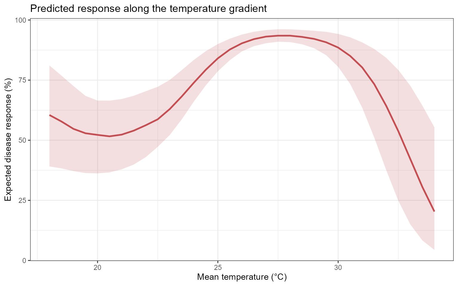
The line represents the central expected response under the fitted model. The ribbon represents uncertainty associated with the fitted model coefficients.

The curve should not be interpreted as a causal dose-response relationship unless the study design and assumptions support that interpretation.

Why sensitivity analysis?

Prediction curves show the expected response along an exposure gradient.

Sensitivity curves describe the local slope of those prediction curves.

For a response function $f(x)$, local sensitivity is conceptually related to:

$$S(x) = \frac{\partial f(x)}{\partial x}$$

where $x$ is the exposure value.

A large absolute sensitivity indicates that the predicted response is changing rapidly at that point of the fitted curve. A sensitivity near zero indicates a locally flat region.

Computing temperature sensitivity

temp_sensitivity <- epi_sensitivity(
  data = response_curve,
  x = "value",
  y = "prediction",
  scenario_var = NULL,
  elasticity = TRUE,
  critical = TRUE,
  k = 3
)

Inspect the resulting columns:

First 10 temperature sensitivity results.

value	prediction	lower	upper	sensitivity	sensitivity_curve_value	elasticity	critical	critical_type	critical_x
18.0	60.4939	39.1146	81.1078	9.2108	37.3974	4.4333	FALSE	NA	NA
18.5	57.7958	38.2991	76.8746	9.1765	41.9971	4.0423	FALSE	NA	NA
19.0	54.7253	37.1710	72.5464	9.0736	46.5625	3.7025	FALSE	NA	NA
19.5	52.9027	36.3691	68.4354	8.9022	51.0593	3.3998	FALSE	NA	NA
20.0	52.2246	36.2260	66.4998	8.6621	55.4532	3.1241	FALSE	NA	NA
20.5	51.6278	36.6358	66.4830	8.3535	59.7100	2.8680	FALSE	NA	NA
21.0	52.3285	37.8897	67.1383	7.9763	63.7953	2.6256	FALSE	NA	NA
21.5	53.9778	39.8684	68.4755	7.5305	67.6749	2.3924	FALSE	NA	NA
22.0	56.2202	42.9446	70.3610	7.0161	71.3144	2.1644	FALSE	NA	NA
22.5	58.6974	47.2438	72.2187	6.4332	74.6796	1.9382	FALSE	NA	NA

Interpreting sensitivity

Positive sensitivity indicates that the expected disease response increases locally as the exposure increases.

Negative sensitivity indicates that the expected disease response decreases locally as the exposure increases.

Values near zero indicate a locally flat region of the model-predicted response curve.

Sensitivity describes the local slope of the prediction curve. It should not automatically be interpreted as disease risk or as a causal effect of changing the exposure.

Visualizing temperature sensitivity

ggplot(
  temp_sensitivity,
  aes(
    x = value,
    y = sensitivity
  )
) +
  geom_hline(
    yintercept = 0,
    color = "grey60",
    linetype = "dashed"
  ) +
  geom_line(
    linewidth = 1,
    color = "#C44E52"
  ) +
  theme_bw() +
  labs(
    x = "Mean temperature (°C)",
    y = "Local sensitivity",
    title = "Sensitivity along the temperature gradient"
  )

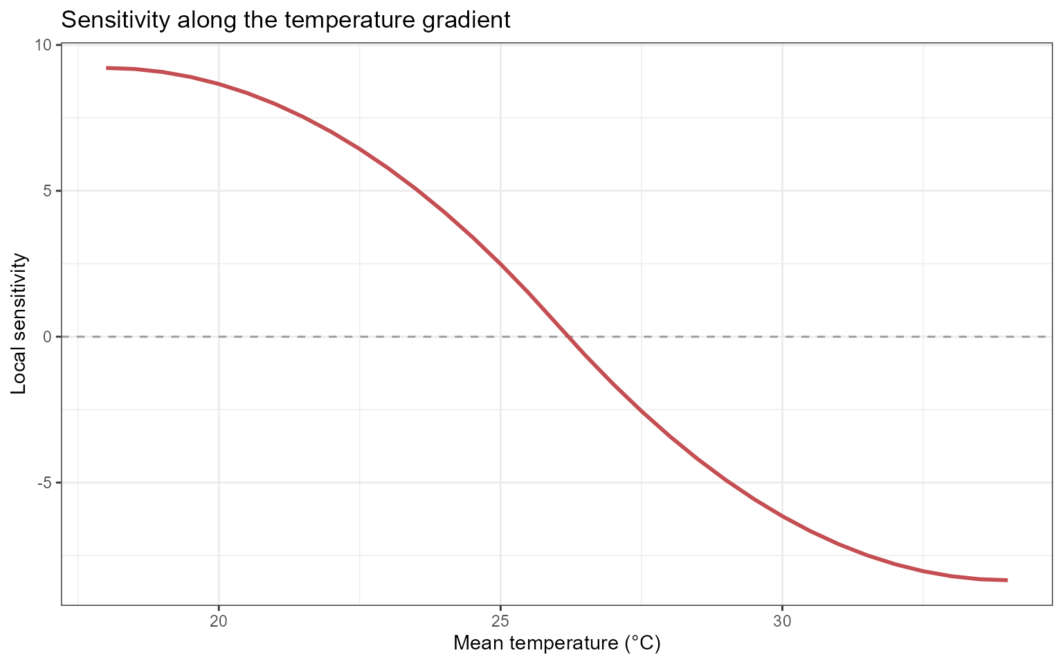
The sign describes the direction of local change, whereas the absolute magnitude describes how rapidly the prediction changes.

Elasticity analysis

What is elasticity?

Sensitivity measures the absolute local rate of change in the predicted response with respect to an exposure.

Elasticity expresses the local response change relative to the current exposure and response scales.

Conceptually, elasticity can be represented as:

$$E(x) = \frac{\partial f(x)}{\partial x} \frac{x}{f(x)}$$

It addresses the question:

What proportional change in the expected disease response is associated with a proportional change in the exposure at this point of the fitted curve?

Elasticity is dimensionless, which can facilitate comparisons across variables measured in different units.

However, elasticity may become unstable when the exposure or predicted response is close to zero. It should be interpreted cautiously in those regions.

Visualizing elasticity

ggplot(
  temp_sensitivity,
  aes(
    x = value,
    y = elasticity
  )
) +
  geom_hline(
    yintercept = 0,
    color = "grey60",
    linetype = "dashed"
  ) +
  geom_line(
    linewidth = 1,
    color = "#4C72B0"
  ) +
  theme_bw() +
  labs(
    x = "Mean temperature (°C)",
    y = "Elasticity",
    title = "Elasticity along the temperature gradient"
  )

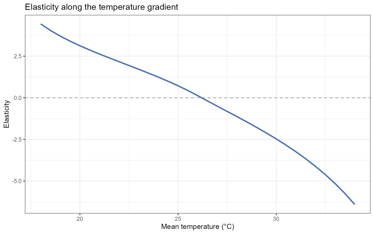
Elasticity should be interpreted together with the underlying prediction and sensitivity curves. A large elasticity value can arise from a small denominator rather than from a large absolute response change.

Identifying critical regions

When:

critical = TRUE

epi_sensitivity() identifies points or regions that satisfy the function’s criterion for comparatively strong local response change.

These locations are model-derived critical regions. They may suggest exposure ranges that deserve closer biological investigation, but they should not automatically be described as biological thresholds.

A biological or management threshold requires additional justification, such as:

• experimental validation;
• an established disease criterion;
• a decision-relevant loss boundary;
• demonstrated management value;
• acceptable classification or forecasting performance.

Extracting critical points

critical_temperature <- temp_sensitivity |>
  dplyr::filter(
    critical
  )

critical_temperature
#>   value prediction    lower  upper sensitivity sensitivity_curve_value
#> 1    26   90.32056 86.96177 93.959   0.4321628                87.67416
#>   elasticity critical critical_type critical_x
#> 1   0.128159     TRUE local_maximum   26.20327

Visualizing critical points

ggplot(
  temp_sensitivity,
  aes(
    x = value,
    y = sensitivity
  )
) +
  geom_hline(
    yintercept = 0,
    color = "grey60",
    linetype = "dashed"
  ) +
  geom_line(
    linewidth = 0.9,
    color = "#C44E52"
  ) +
  geom_point(
    data = critical_temperature,
    color = "#B22222",
    size = 2.8
  ) +
  theme_bw() +
  labs(
    x = "Mean temperature (°C)",
    y = "Local sensitivity",
    title = "Model-derived critical regions along the temperature gradient"
  )

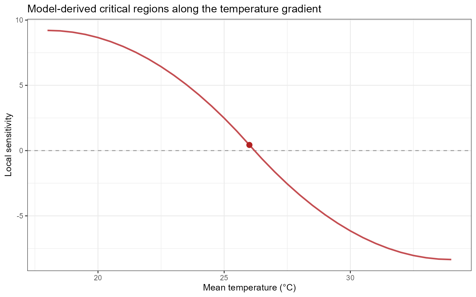
The highlighted points indicate comparatively strong local changes according to the criterion used by epi_sensitivity(). They do not, by themselves, establish biologically validated thresholds.

Comparing environmental drivers

Sensitivity analyses can also be conducted for rainfall and leaf wetness.

The following examples evaluate one exposure at a time while holding the other environmental variables constant.

Rainfall sensitivity

Generating a rainfall gradient

rain_range <- simulate_ranges(
  periods = periods,
  vary = list(
    tmean = 25,
    wetness = 10,
    rain = seq(
      0,
      15,
      by = 0.5
    )
  ),
  scenario_type = "grid",
  scenario_var = "rain"
)

Predicting rainfall scenarios

Sample-level predictions are requested so that sensitivity can be evaluated across uncertainty realizations:

rain_predictions <- simulate_scenarios(
  fit = fit,
  scenarios = rain_range,
  data = epi_data,
  uncertainty = TRUE,
  output = "samples",
  n_samples = 100,
  seed = 123
)

Computing rainfall sensitivity

sens_rain <- epi_sensitivity(
  data = rain_predictions,
  x = "rain",
  y = "prediction",
  scenario_var = "sample",
  elasticity = TRUE,
  critical = TRUE,
  method = "finite",
  k = 3
)

Leaf wetness sensitivity

Generating a leaf wetness gradient

wetness_range <- simulate_ranges(
  periods = periods,
  vary = list(
    tmean = 25,
    rain = 5,
    wetness = seq(
      0,
      24,
      by = 0.5
    )
  ),
  scenario_type = "grid",
  scenario_var = "wetness"
)

Predicting leaf wetness scenarios

wetness_predictions <- simulate_scenarios(
  fit = fit,
  scenarios = wetness_range,
  data = epi_data,
  uncertainty = TRUE,
  output = "samples",
  n_samples = 100,
  seed = 456
)

Computing leaf wetness sensitivity

sens_wetness <- epi_sensitivity(
  data = wetness_predictions,
  x = "wetness",
  y = "prediction",
  scenario_var = "sample",
  elasticity = TRUE,
  critical = TRUE,
  method = "finite",
  k = 3
)

Combining sensitivity results

Rainfall and leaf wetness are measured on different scales. Therefore, they should not be placed on a shared exposure axis without preserving their original units.

Create a common exposure-value column and retain the variable identifier:

sens_rain_plot <- sens_rain |>
  dplyr::mutate(
    variable = "Rainfall",
    exposure_value = rain
  )

sens_wetness_plot <- sens_wetness |>
  dplyr::mutate(
    variable = "Leaf wetness",
    exposure_value = wetness
  )

combined_sensitivity <- dplyr::bind_rows(
  sens_rain_plot,
  sens_wetness_plot
)

Visualizing uncertainty realizations

ggplot(
  combined_sensitivity,
  aes(
    x = exposure_value,
    y = sensitivity,
    group = sample
  )
) +
  geom_hline(
    yintercept = 0,
    color = "grey60",
    linetype = "dashed"
  ) +
  geom_line(
    alpha = 0.10,
    linewidth = 0.35,
    color = "#4C72B0"
  ) +
  facet_wrap(
    vars(
      variable
    ),
    scales = "free_x"
  ) +
  theme_bw() +
  labs(
    x = "Exposure value",
    y = "Local sensitivity",
    title = "Sensitivity across environmental gradients"
  )

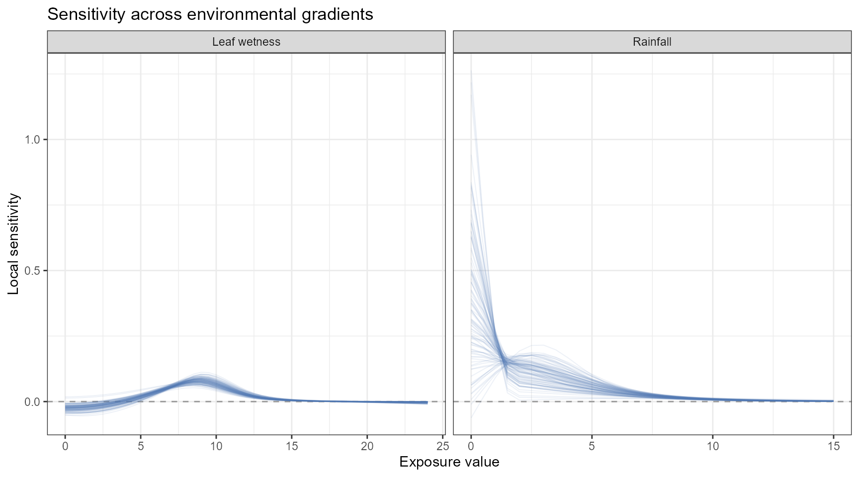
Each line represents one uncertainty realization. The collection of lines shows how coefficient uncertainty propagates into the estimated sensitivity curves.

If the sample identifier returned by simulate_scenarios() has a different column name, replace:

group = sample

with the corresponding sample-identification column.

Summarizing sensitivity uncertainty

Sample-level sensitivity results can be summarized at each exposure value.

sensitivity_summary <- combined_sensitivity |>
  dplyr::group_by(
    variable,
    exposure_value
  ) |>
  dplyr::summarise(
    sensitivity_median = stats::median(
      sensitivity,
      na.rm = TRUE
    ),
    sensitivity_lower = stats::quantile(
      sensitivity,
      probs = 0.025,
      na.rm = TRUE
    ),
    sensitivity_upper = stats::quantile(
      sensitivity,
      probs = 0.975,
      na.rm = TRUE
    ),
    .groups = "drop"
  )

Inspect the summaries:

First 10 summarized sensitivity estimates.

variable	exposure_value	sensitivity_median	sensitivity_lower	sensitivity_upper
Leaf wetness	0.0	-0.0241	-0.0455	-0.0053
Leaf wetness	0.5	-0.0236	-0.0453	-0.0047
Leaf wetness	1.0	-0.0225	-0.0449	-0.0037
Leaf wetness	1.5	-0.0205	-0.0432	-0.0019
Leaf wetness	2.0	-0.0175	-0.0406	0.0006
Leaf wetness	2.5	-0.0136	-0.0366	0.0038
Leaf wetness	3.0	-0.0086	-0.0312	0.0078
Leaf wetness	3.5	-0.0028	-0.0244	0.0125
Leaf wetness	4.0	0.0036	-0.0165	0.0180
Leaf wetness	4.5	0.0107	-0.0074	0.0241

Visualizing summarized sensitivity

ggplot(
  sensitivity_summary,
  aes(
    x = exposure_value,
    y = sensitivity_median
  )
) +
  geom_hline(
    yintercept = 0,
    color = "grey60",
    linetype = "dashed"
  ) +
  geom_ribbon(
    aes(
      ymin = sensitivity_lower,
      ymax = sensitivity_upper
    ),
    fill = "#4C72B0",
    alpha = 0.18
  ) +
  geom_line(
    linewidth = 0.9,
    color = "#4C72B0"
  ) +
  facet_wrap(
    vars(
      variable
    ),
    scales = "free_x"
  ) +
  theme_bw() +
  labs(
    x = "Exposure value",
    y = "Local sensitivity",
    title = "Summarized sensitivity across environmental gradients"
  )

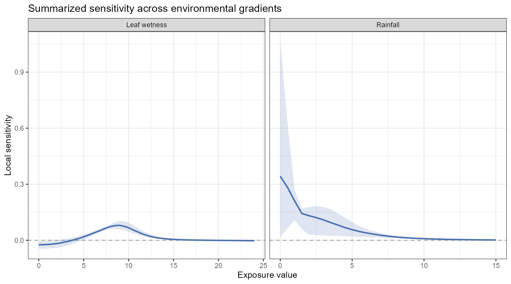
The uncertainty interval describes uncertainty propagated from the fitted model into the sensitivity calculation. It does not include uncertainty in the scenario values or additional observation-level variability.

Comparing sensitivity across variables

Absolute sensitivity values depend on the units of both the exposure and the predicted response.

For example:

• temperature is measured in degrees Celsius;
• rainfall is measured in millimeters;
• leaf wetness is measured in its recorded unit.

Consequently, the numerical magnitudes of raw sensitivity should not be compared directly across variables without considering their units and scales.

Elasticity can facilitate proportional comparisons because it is dimensionless. However, elasticity can be unstable near zero exposure or zero predicted response.

A defensible comparison should therefore consider:

• sensitivity;
• elasticity;
• predicted disease level;
• uncertainty;
• observed exposure support;
• biological plausibility;
• the units and feasible range of each exposure.

Decision-support interpretation

Sensitivity analysis can help identify model-derived regions that merit closer attention, but it does not automatically define a management rule.

Potential applications include:

• identifying exposure ranges associated with rapid predicted response change;
• prioritizing environmental monitoring;
• identifying candidate regions for experimental validation;
• informing the construction of warning criteria;
• comparing sensitivity across environmental gradients;
• examining climate or management scenarios;
• supporting disease-forecasting research.

A decision-support interpretation should combine sensitivity with additional information, including:

• the absolute predicted disease response;
• uncertainty in the prediction and sensitivity;
• the frequency of the exposure condition;
• exposure values supported by the observed data;
• biological feasibility;
• intervention timing;
• management costs;
• potential yield or economic losses;
• consequences of false-positive and false-negative decisions.

High sensitivity is not automatically high disease. Sensitivity describes the local slope of the predicted response curve. A region can have high sensitivity but a moderate predicted response, or high predicted disease but low sensitivity if the response curve has reached a plateau.

Example interpretation

Suppose the temperature sensitivity analysis indicates:

• relatively small local changes below 20 °C;
• the largest positive sensitivity between 24 and 28 °C;
• decreasing sensitivity above 30 °C.

Under the fitted model, the expected disease response changes most rapidly along the 24–28 °C portion of the evaluated temperature gradient.

This region may deserve closer monitoring or biological investigation. However, high sensitivity alone does not establish a management threshold.

A management interpretation should also consider:

• the predicted disease level in that region;
• uncertainty around the sensitivity estimates;
• whether temperatures in that interval are common in the target system;
• whether the exposure can be modified;
• whether an intervention can be applied in time;
• the expected yield and economic consequences;
• the cost and effectiveness of the intervention.

Interpretation checklist

Before reporting sensitivity or elasticity results, verify:

1. which response family and link were fitted;
2. which environmental variable was varied;
3. which variables were held constant;
4. which lag periods were represented in the scenarios;
5. whether the evaluated gradient is supported by the observed data;
6. whether the disease response was analyzed as a proportion or percentage;
7. whether uncertainty samples were propagated;
8. how the sensitivity derivative was estimated;
9. how critical regions were defined;
10. whether the result is being interpreted as a modeled association or as a validated decision threshold.

Summary

This section demonstrated how EpiExposure can be used to examine local changes along model-predicted response curves.

The sensitivity workflow consists of:

controlled exposure gradient
            ↓
predicted disease-response curve
            ↓
local sensitivity
            ↓
elasticity
            ↓
model-derived critical regions

The principal tools are:

• simulate_ranges() for creating controlled exposure gradients;
• simulate_scenarios() for predicting responses along those gradients;
• epi_sensitivity() for calculating sensitivity, elasticity, and critical regions.

Sensitivity analysis complements the effect summaries introduced in the Understanding Effects section

Lag-specific and period-specific effects describe the fitted exposure-lag association, whereas sensitivity describes how rapidly a predicted response changes along a selected environmental gradient.

Sensitivity and elasticity are model-derived quantities. Their use in decision support requires biological interpretation, uncertainty assessment, and decision criteria appropriate to the pathosystem.

Next steps

The next section, Simulation and Prediction, expands from controlled one-variable gradients to complete hypothetical exposure profiles and multivariable scenarios.

It introduces:

• simulate_exposures() for generating complete chronological profiles;
• simulate_ranges() for constructing candidate exposure combinations;
• simulate_scenarios() for predicting across scenario grids;
• predict_outcomes() for complete exposure profiles;
• compare_exposures() for comparing environmental profiles;
• compare_predictions() for comparing their expected disease outcomes.

These tools allow researchers to investigate exposure timing, construct alternative environmental profiles, propagate parameter uncertainty, and compare model-based disease predictions.