Yield and Economic Losses

Ricardo G. Tomáz

Introduction

Predicted disease intensity alone does not fully describe the potential agronomic consequences of an epidemic.

In many pathosystems, researchers also want to estimate how the predicted disease response may translate into reduced crop yield and economic losses.

EpiExposure connects three modeling stages:

1. environmental exposure profiles;
2. expected disease outcomes from the fitted DLNM;
3. user-defined disease-yield and economic relationships.

This section demonstrates how scenario predictions can be translated into:

• expected remaining yield;
• yield loss;
• proportional yield loss;
• economic loss;
• comparisons across production scenarios.

What you will learn. This tutorial shows how to convert predicted disease outcomes into yield and economic losses, evaluate sensitivity to attainable yield, and compare the agronomic consequences of alternative environmental scenarios.

Yield and economic losses are not estimated by the DLNM alone. They depend on additional assumptions supplied by the user, including the disease-yield relationship, attainable yield, commodity price, and unit conversions.

The resulting quantities are model-based projections under those assumptions. They should not automatically be interpreted as observed losses or causal effects.

Preparing the epidemiological model

This section uses the same example dataset and DLNM specification introduced in the previous tutorials.

library(EpiExposure)
library(ggplot2)

data("epi_data")

Define the exposure-lag structures:

cb <- define_exposures(
  data = epi_data,
  vars = c(
    "tmean",
    "rain",
    "wetness"
  ),
  max_lag = 85,
  df_var = 3,
  df_lag = 2
)

Build the epidemic-level design:

dat <- build_design(
  data = epi_data,
  cb_templates = cb
)

Prepare the disease response:

dat <- prepare_response(
  data = dat,
  response = "y",
  family = "beta"
)

Fit the DLNM:

fit <- fit_epidlnm(
  data = dat,
  model_engine = "glmmTMB",
  family = "beta",
  random_effect = NULL,
  epiexposure_spec = attr(
    cb,
    "spec"
  )
)

The fitted model is now used to predict disease responses across environmental scenarios and translate those predictions into agronomic and economic quantities.

Translating disease predictions into losses

Disease and yield scales

The fitted Beta model returns predicted disease outcomes on a proportion scale between 0 and 1. However, the damage function used in this example was defined using disease severity in percentage points.

Therefore, predictions and uncertainty limits are converted from proportions to percentages before the yield-loss relationship is applied:

$$D_{\%} = 100D_{\mathrm{proportion}}$$

This conversion is specific to the damage function used in the example. Users must verify the disease scale associated with their own slope and intercept parameters.

Generating disease scenarios

Define biologically meaningful lag periods:

periods <- define_periods(
  max_lag = 85,
  cuts = c(
    20,
    40,
    60
  ),
  prefix = "Period"
)

Generate a scenario grid in which rainfall varies continuously across selected temperature and leaf wetness conditions:

range_losses <- simulate_ranges(
  periods = periods,
  vary = list(
    tmean = c(
      20,
      34
    ),
    rain = seq(
      0,
      15,
      by = 1
    ),
    wetness = c(
      2,
      10
    )
  ),
  scenario_type = "grid",
  scenario_var = "rain"
)

The fine rainfall sequence provides a smooth grid for visualizing the modeled disease and loss relationships. It should not be interpreted as additional observed information.

Predict expected disease outcomes and propagate coefficient uncertainty:

scenarios_losses <- simulate_scenarios(
  fit = fit,
  scenarios = range_losses,
  data = epi_data,
  uncertainty = TRUE,
  output = "summary",
  n_samples = 5,
  seed = 123
)

The Beta-model predictions are proportions. Convert the central estimates and interval limits to percentage points because the damage coefficient used below was defined for percentage disease severity:

scenarios_losses$prediction <- (
  scenarios_losses$prediction * 100
)

scenarios_losses$prediction_lower <- (
  scenarios_losses$prediction_lower * 100
)

scenarios_losses$prediction_upper <- (
  scenarios_losses$prediction_upper * 100
)

Match the damage-function scale. Multiplication by 100 is appropriate only because this example applies a damage coefficient defined per percentage point of disease severity. Do not perform this conversion when the damage function was estimated directly from proportions.

Simulating yield and economic losses

A single damage function

Suppose expected yield under disease is described by the linear relationship:

$$Y_{\mathrm{disease}} = a - bD$$

where:

• $Y_{\mathrm{disease}}$ is expected yield under disease;
• $D$ is disease severity in percentage points;
• $a$ is the intercept of the damage function;
• $b$ is the yield reduction per percentage point of disease severity.

For this example:

intercept = 9691.0
slope = 49.3

Thus, each additional percentage point of predicted severity is associated with 49.3 kilograms per percentage point (kg/p.p) under the specified damage relationship.

Estimate yield and economic losses over attainable yields ranging from 4,000 to 12,000:

losses <- simulate_losses(
  data = scenarios_losses,
  lower = "prediction_lower",
  upper = "prediction_upper",
  y = "prediction",
  slope = 49.3,
  parameter_mode = "values",
  intercept = 9691.0,
  attainable_yield = seq(
    4000,
    10000,
    by = 50
  ),
  price = 300
)

In this example, price = 300 represents a commodity price of 300 USD per metric ton. Because yield loss is expressed in kg ha⁻¹, simulate_losses() internally converts yield loss from kilograms to metric tons before calculating economic loss:

$$L_{\mathrm{economic}} = \left( \frac{L_{\mathrm{yield}}}{1000} \right) P$$

where $L_{\mathrm{yield}}$ is yield loss in kg ha⁻¹, $P$ is commodity price in USD t⁻¹, and $L_{\mathrm{economic}}$ is economic loss in USD ha⁻¹.

Inspect the resulting columns:

names(
  losses
)
#>  [1] "scenario"          "scenario_point"    "tmean"            
#>  [4] "rain"              "wetness"           "prediction"       
#>  [7] "prediction_sd"     "prediction_lower"  "prediction_upper" 
#> [10] ".loss_row_id"      ".sim"              "slope_sim"        
#> [13] "intercept_sim"     "rand_eff"          "ref_yield"        
#> [16] "att_yield"         "price"             "y_used"           
#> [19] "y_lower"           "y_upper"           "yl_prop_raw"      
#> [22] "yl_capped"         "pred_yield"        "rl_prop"          
#> [25] "rl_pct"            "yl_prop"           "yl_pct"           
#> [28] "ap_yield"          "yield_loss"        "econ_loss"        
#> [31] "yl_prop_raw_lower" "yl_prop_raw_upper" "pred_yield_lower" 
#> [34] "pred_yield_upper"  "rl_prop_lower"     "rl_prop_upper"    
#> [37] "rl_pct_lower"      "rl_pct_upper"      "yl_prop_lower"    
#> [40] "yl_prop_upper"     "yl_pct_lower"      "yl_pct_upper"     
#> [43] "ap_yield_lower"    "ap_yield_upper"    "yield_loss_lower" 
#> [46] "yield_loss_upper"  "econ_loss_lower"   "econ_loss_upper"  
#> [49] "yl_capped_lower"   "yl_capped_upper"

scenario	scenario_point	tmean	rain	wetness	prediction	prediction_sd	prediction_lower	prediction_upper	.loss_row_id	.sim	slope_sim	intercept_sim	rand_eff	ref_yield	att_yield	price	y_used	y_lower	y_upper	yl_prop_raw	yl_capped	pred_yield	rl_prop	rl_pct	yl_prop	yl_pct	ap_yield	yield_loss	econ_loss	yl_prop_raw_lower	yl_prop_raw_upper	pred_yield_lower	pred_yield_upper	rl_prop_lower	rl_prop_upper	rl_pct_lower	rl_pct_upper	yl_prop_lower	yl_prop_upper	yl_pct_lower	yl_pct_upper	ap_yield_lower	ap_yield_upper	yield_loss_lower	yield_loss_upper	econ_loss_lower	econ_loss_upper	yl_capped_lower	yl_capped_upper
RAIN_s1	1	20	0	2	0.628	0.002	0.61	1.107	1	1	49.3	9691	0	9691	4000	300	0.628	0.61	1.107	0.003	FALSE	9660.016	0.997	99.68	0.003	0.32	3987.211	12.789	3.837	0.003	0.006	9636.405	9660.944	0.994	0.997	99.437	99.69	0.003	0.006	0.31	0.563	3977.466	3987.594	12.406	22.534	3.722	6.760	FALSE	FALSE
RAIN_s1	1	20	0	2	0.628	0.002	0.61	1.107	1	1	49.3	9691	0	9691	4050	300	0.628	0.61	1.107	0.003	FALSE	9660.016	0.997	99.68	0.003	0.32	4037.051	12.949	3.885	0.003	0.006	9636.405	9660.944	0.994	0.997	99.437	99.69	0.003	0.006	0.31	0.563	4027.184	4037.439	12.561	22.816	3.768	6.845	FALSE	FALSE
RAIN_s1	1	20	0	2	0.628	0.002	0.61	1.107	1	1	49.3	9691	0	9691	4100	300	0.628	0.61	1.107	0.003	FALSE	9660.016	0.997	99.68	0.003	0.32	4086.891	13.109	3.933	0.003	0.006	9636.405	9660.944	0.994	0.997	99.437	99.69	0.003	0.006	0.31	0.563	4076.902	4087.284	12.716	23.098	3.815	6.929	FALSE	FALSE
RAIN_s1	1	20	0	2	0.628	0.002	0.61	1.107	1	1	49.3	9691	0	9691	4150	300	0.628	0.61	1.107	0.003	FALSE	9660.016	0.997	99.68	0.003	0.32	4136.731	13.269	3.981	0.003	0.006	9636.405	9660.944	0.994	0.997	99.437	99.69	0.003	0.006	0.31	0.563	4126.621	4137.129	12.871	23.379	3.861	7.014	FALSE	FALSE
RAIN_s1	1	20	0	2	0.628	0.002	0.61	1.107	1	1	49.3	9691	0	9691	4200	300	0.628	0.61	1.107	0.003	FALSE	9660.016	0.997	99.68	0.003	0.32	4186.572	13.428	4.029	0.003	0.006	9636.405	9660.944	0.994	0.997	99.437	99.69	0.003	0.006	0.31	0.563	4176.339	4186.974	13.026	23.661	3.908	7.098	FALSE	FALSE
RAIN_s1	1	20	0	2	0.628	0.002	0.61	1.107	1	1	49.3	9691	0	9691	4250	300	0.628	0.61	1.107	0.003	FALSE	9660.016	0.997	99.68	0.003	0.32	4236.412	13.588	4.076	0.003	0.006	9636.405	9660.944	0.994	0.997	99.437	99.69	0.003	0.006	0.31	0.563	4226.057	4236.819	13.181	23.943	3.954	7.183	FALSE	FALSE
RAIN_s1	1	20	0	2	0.628	0.002	0.61	1.107	1	1	49.3	9691	0	9691	4300	300	0.628	0.61	1.107	0.003	FALSE	9660.016	0.997	99.68	0.003	0.32	4286.252	13.748	4.124	0.003	0.006	9636.405	9660.944	0.994	0.997	99.437	99.69	0.003	0.006	0.31	0.563	4275.776	4286.664	13.336	24.224	4.001	7.267	FALSE	FALSE
RAIN_s1	1	20	0	2	0.628	0.002	0.61	1.107	1	1	49.3	9691	0	9691	4350	300	0.628	0.61	1.107	0.003	FALSE	9660.016	0.997	99.68	0.003	0.32	4336.092	13.908	4.172	0.003	0.006	9636.405	9660.944	0.994	0.997	99.437	99.69	0.003	0.006	0.31	0.563	4325.494	4336.509	13.491	24.506	4.047	7.352	FALSE	FALSE
RAIN_s1	1	20	0	2	0.628	0.002	0.61	1.107	1	1	49.3	9691	0	9691	4400	300	0.628	0.61	1.107	0.003	FALSE	9660.016	0.997	99.68	0.003	0.32	4385.932	14.068	4.220	0.003	0.006	9636.405	9660.944	0.994	0.997	99.437	99.69	0.003	0.006	0.31	0.563	4375.212	4386.354	13.646	24.788	4.094	7.436	FALSE	FALSE
RAIN_s1	1	20	0	2	0.628	0.002	0.61	1.107	1	1	49.3	9691	0	9691	4450	300	0.628	0.61	1.107	0.003	FALSE	9660.016	0.997	99.68	0.003	0.32	4435.772	14.228	4.268	0.003	0.006	9636.405	9660.944	0.994	0.997	99.437	99.69	0.003	0.006	0.31	0.563	4424.931	4436.199	13.801	25.069	4.140	7.521	FALSE	FALSE

Visualizing the loss scenarios

plot_losses() can display the yield and economic consequences across the environmental scenario grid.

losses_plot <- plot_losses(
  data = losses,
  x = "rain",
  y = "att_yield",
  facet = c(
    "tmean",
    "wetness"
  ),
  type = "heatmap",
  x_breaks = seq(
    0,
    15,
    by = 3
  ),
  y_breaks = seq(
    4000,
    10000,
    by = 2000
  ),
  x_label = "Daily precipitation (mm)",
  nrow = 2,
  facet_ncol = 4
)

losses_plot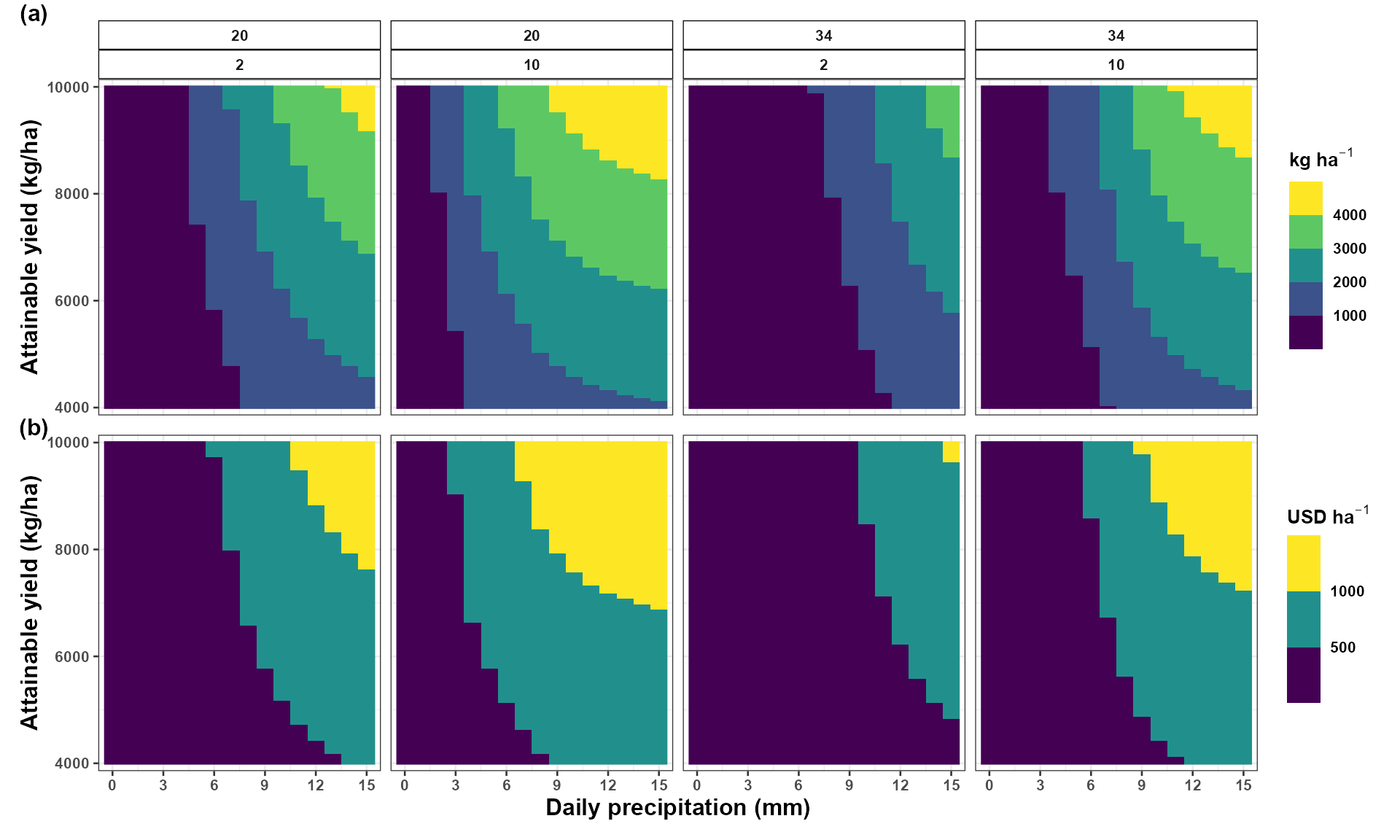

The heatmap summarizes the complete modeling chain:

rainfall, temperature, and leaf wetness scenarios
                         ↓
predicted disease severity
                         ↓
linear damage relationship
                         ↓
estimated yield and economic losses

Rainfall should not be interpreted in isolation because the panels also represent different temperature and leaf wetness conditions.

Sensitivity to damage-function parameters

Damage-function parameters may vary among studies, cultivars, production systems, or experimental conditions. simulate_losses() can evaluate multiple parameter values to show how agronomic conclusions depend on the selected disease-yield relationship.

The following example compares two parameter combinations:

Damage relationship 1: intercept = 9691.0, slope = 49.3
Damage relationship 2: intercept = 12000, slope = 80

losses_sensitivity <- simulate_losses(
  data = scenarios_losses,
  lower = "prediction_lower",
  upper = "prediction_upper",
  y = "prediction",
  slope = c(
    49.3,
    80
  ),
  parameter_mode = "values",
  intercept = c(
    9691.0,
    12000
  ),
  attainable_yield = seq(
    4000,
    10000,
    by = 50
  ),
  price = 300
)

The parameter combinations represent alternative damage relationships rather than uncertainty intervals around one damage function. Their scientific source and interpretation should be stated explicitly in a real analysis.

Visualize the modeled relationship between rainfall and predicted yield for a selected attainable yield:

plot_losses(
  data = losses_sensitivity,
  x = "rain",
  y = "att_yield",
  facet = c(
    "tmean",
    "wetness"
  ),
  type = "regression",
  reg_y = "ap_yield",
  att_yield = 10000,
  x_breaks = seq(
    0,
    15,
    by = 3
  ),
  x_label = "Daily precipitation (mm)"
)

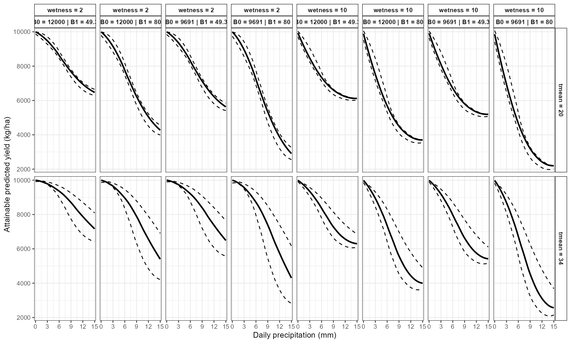
This sensitivity analysis helps determine whether the agronomic conclusions remain similar across plausible disease-yield relationships.

Interpreting the loss results

The outputs combine assumptions from several stages:

1. the fitted exposure-lag-response model;
2. the simulated environmental scenarios;
3. the conversion of disease predictions into percentage severity;
4. the selected slope and intercept;
5. the attainable-yield range;
6. the commodity price.

The lower and upper disease-prediction limits are transformed through the damage relationship to obtain corresponding loss limits. This interval transformation does not automatically represent full draw-by-draw propagation of every source of uncertainty.

The resulting limits do not automatically include uncertainty in:

• slope;
• intercept;
• attainable yield;
• commodity price;
• environmental scenario assumptions.

The second analysis varies slope and intercept explicitly, but these values are alternative parameter combinations rather than random draws from an estimated joint parameter distribution.

Practical applications

When supported by appropriate data and assumptions, yield and economic loss simulations can help researchers:

• translate disease predictions into agronomic units;
• compare hypothetical environmental scenarios;
• examine sensitivity to attainable yield;
• evaluate sensitivity to commodity price;
• identify scenarios associated with larger modeled losses;
• connect disease forecasting with production consequences;
• explore assumptions used in management or climate scenarios.

These applications remain conditional on the fitted epidemiological model and the disease-yield relationship supplied by the user.

Reporting checklist

When reporting loss estimates, specify:

1. the response family and disease scale;
2. the fitted DLNM specification;
3. the environmental profiles or scenarios;
4. the disease-yield equation;
5. the source and units of the slope and intercept;
6. the range and units of attainable yield;
7. the commodity price and price unit;
8. any conversion between kilograms and metric tons;
9. the uncertainty sources that were propagated;
10. whether the results are associational projections or causal estimates.

Summary

This section demonstrated how EpiExposure connects exposure-lag-response modeling with agronomic and economic outcomes.

The workflow is:

complete exposure profiles
            ↓
fitted DLNM
            ↓
expected disease response
            ↓
user-supplied disease-yield relationship
            ↓
expected remaining yield
            ↓
yield loss
            ↓
economic loss

The DLNM describes the modeled association between environmental profiles and disease. The damage function translates predicted disease into expected yield, and commodity price translates yield loss into economic units.

Each stage introduces assumptions that should be documented and evaluated through sensitivity analysis.

Next steps

The next section focuses on model selection and ensemble prediction.

Topics include:

• find_bestfit();
• model ranking;
• cross-validation;
• ensemble_bestfit().

These tools help compare candidate exposure-lag specifications and evaluate their predictive performance.