Packages

library(dplyr)
library(tidyr)
library(ggplot2)
library(metafor)
library(gsheet)
library(tidytext)
library(cowplot)

gs_url <- "https://docs.google.com/spreadsheets/d/1i7f61MP5efJclMLpQWgh9k3iTyX7Xgvj/edit?gid=1609934999#gid=1609934999"

diseases <- c("poli","comum","branca","cercos","turc","diplo","antrac","bipol")
thr_present <- 1.6  

price <- 200      
cost  <- 80      

dat <- gsheet2tbl(gs_url) %>%
  mutate(
    application = tolower(trimws(application)),
    season      = factor(tolower(trimws(season)), levels = c("first","second")),
    location    = trimws(location),
    trial       = paste(year, location, season, sep = "_")
  )

stopifnot(all(c("check","treated") %in% dat$application))

dat$poli[is.na(dat$poli)] <- 0
dat$comum[is.na(dat$comum)] <- 0
dat$branca[is.na(dat$branca)] <- 0
dat$cercos[is.na(dat$cercos)] <- 0
dat$turc[is.na(dat$turc)] <- 0
dat$diplo[is.na(dat$diplo)] <- 0
dat$antrac[is.na(dat$antrac)] <- 0
dat$bipol[is.na(dat$bipol)] <- 0

hyb_app <- dat %>%
  group_by(trial, year, location, season, hybrid, application) %>%
  summarise(
    yield = mean(yield, na.rm = TRUE),
    across(all_of(diseases), mean, na.rm = TRUE),
    .groups = "drop"
  )

hyb_app

hyb_diff <- hyb_app %>%
  pivot_wider(
    names_from  = application,
    values_from = c(yield, all_of(diseases))
  ) %>%
  filter(!is.na(yield_check) & !is.na(yield_treated)) %>%
  mutate(d_yld = yield_treated - yield_check)

es <- hyb_diff %>%
  rowwise() %>%
  mutate(sev_sum_check = sum(c_across(all_of(paste0(diseases, "_check"))), na.rm = TRUE)) %>%
  ungroup() %>%
  group_by(trial, year, location, season) %>%
  summarise(
    yi        = mean(d_yld, na.rm = TRUE),
    vi        = var(d_yld, na.rm = TRUE) / sum(!is.na(d_yld)),
    m_hybrids = sum(!is.na(d_yld)),
    sev_sum   = mean(sev_sum_check, na.rm = TRUE),
    .groups   = "drop"
  ) %>%
  mutate(
    pressure = factor(
      ifelse(sev_sum > thr_present, "Disease present (>2%)", "Disease absent (≤2%)"),
      levels = c("Disease absent (≤2%)", "Disease present (>2%)")
    )
  ) %>%
  filter(is.finite(vi), vi > 0, m_hybrids >= 2)# %>% 
  #filter(!trial == "2019_Pato Branco_first")

es %>% 
  filter(sev_sum > 0.1) %>% 
  summarise(
    mean = mean(sev_sum),
    min = min(sev_sum),
    max = max(sev_sum),
    median = median(sev_sum)
  )

m0 <- rma(yi, vi, data = es, method = "REML")
m0

Random-Effects Model (k = 19; tau^2 estimator: REML)

tau^2 (estimated amount of total heterogeneity): 0.3904 (SE = 0.1385)
tau (square root of estimated tau^2 value):      0.6249
I^2 (total heterogeneity / total variability):   95.53%
H^2 (total variability / sampling variability):  22.37

Test for Heterogeneity:
Q(df = 18) = 264.1120, p-val < .0001

Model Results:

estimate      se    zval    pval   ci.lb   ci.ub     
  0.4456  0.1480  3.0117  0.0026  0.1556  0.7357  ** 

---
Signif. codes:  0 '***' 0.001 '**' 0.01 '*' 0.05 '.' 0.1 ' ' 1

mP <- rma(yi, vi, mods = ~ pressure, data = es, method = "REML")
mP

Mixed-Effects Model (k = 19; tau^2 estimator: REML)

tau^2 (estimated amount of residual heterogeneity):     0.2623 (SE = 0.0985)
tau (square root of estimated tau^2 value):             0.5122
I^2 (residual heterogeneity / unaccounted variability): 93.36%
H^2 (unaccounted variability / sampling variability):   15.06
R^2 (amount of heterogeneity accounted for):            32.81%

Test for Residual Heterogeneity:
QE(df = 17) = 191.4251, p-val < .0001

Test of Moderators (coefficient 2):
QM(df = 1) = 9.0906, p-val = 0.0026

Model Results:

                               estimate      se    zval    pval    ci.lb 
intrcpt                          0.0926  0.1692  0.5469  0.5844  -0.2392 
pressureDisease present (>2%)    0.7430  0.2464  3.0151  0.0026   0.2600 
                                ci.ub     
intrcpt                        0.4243     
pressureDisease present (>2%)  1.2260  ** 

---
Signif. codes:  0 '***' 0.001 '**' 0.01 '*' 0.05 '.' 0.1 ' ' 1

mP2 <- rma(yi, vi, mods = ~ season, data = es, method = "REML")
mP2

Mixed-Effects Model (k = 19; tau^2 estimator: REML)

tau^2 (estimated amount of residual heterogeneity):     0.4033 (SE = 0.1470)
tau (square root of estimated tau^2 value):             0.6351
I^2 (residual heterogeneity / unaccounted variability): 95.62%
H^2 (unaccounted variability / sampling variability):   22.85
R^2 (amount of heterogeneity accounted for):            0.00%

Test for Residual Heterogeneity:
QE(df = 17) = 259.2878, p-val < .0001

Test of Moderators (coefficient 2):
QM(df = 1) = 0.5011, p-val = 0.4790

Model Results:

              estimate      se    zval    pval    ci.lb   ci.ub    
intrcpt         0.3316  0.2205  1.5040  0.1326  -0.1005  0.7637    
seasonsecond    0.2133  0.3013  0.7079  0.4790  -0.3772  0.8037    

---
Signif. codes:  0 '***' 0.001 '**' 0.01 '*' 0.05 '.' 0.1 ' ' 1

es$pressure <- factor(es$pressure,
                      levels = c("Disease absent (≤2%)", "Disease present (>2%)"))

newP <- data.frame(pressure = levels(es$pressure))

X_P <- model.matrix(~ pressure, data = newP)[, -1, drop = FALSE]  # one column

pred_P <- predict(mP, newmods = X_P)

pred_tab <- data.frame(
  pressure = newP$pressure,
  gain_hat = pred_P$pred,
  se       = pred_P$se,
  ci_lb    = pred_P$ci.lb,
  ci_ub    = pred_P$ci.ub
)

pred_tab

es$season <- factor(es$season,
                      levels = c("first", "second"))

newP <- data.frame(season = levels(es$season))

X_P <- model.matrix(~ season, data = newP)[, -1, drop = FALSE]  # one column

pred_P <- predict(mP2, newmods = X_P)

pred_tab2 <- data.frame(
  season = newP$season,
  gain_hat = pred_P$pred,
  se       = pred_P$se,
  ci_lb    = pred_P$ci.lb,
  ci_ub    = pred_P$ci.ub
)

pred_tab2

hyb_lnr <- hyb_diff %>%
  filter(yield_check > 0, yield_treated > 0) %>%
  mutate(lnRR = log(yield_treated / yield_check))

es_lnr <- hyb_lnr %>%
  group_by(trial, year, location, season) %>%
  summarise(
    yi = mean(lnRR, na.rm = TRUE),
    vi = var(lnRR, na.rm = TRUE) / sum(!is.na(lnRR)),
    .groups = "drop"
  ) %>%
  filter(is.finite(vi), vi > 0) %>%
  left_join(es %>% select(trial, pressure), by = "trial")

es_lnr

mP_lnr <- rma(yi, vi, mods = ~ pressure, data = es_lnr, method = "REML")

mP_lnr

Mixed-Effects Model (k = 19; tau^2 estimator: REML)

tau^2 (estimated amount of residual heterogeneity):     0.0042 (SE = 0.0016)
tau (square root of estimated tau^2 value):             0.0645
I^2 (residual heterogeneity / unaccounted variability): 93.11%
H^2 (unaccounted variability / sampling variability):   14.52
R^2 (amount of heterogeneity accounted for):            35.21%

Test for Residual Heterogeneity:
QE(df = 17) = 163.7050, p-val < .0001

Test of Moderators (coefficient 2):
QM(df = 1) = 9.5946, p-val = 0.0020

Model Results:

                               estimate      se    zval    pval    ci.lb 
intrcpt                          0.0122  0.0214  0.5692  0.5692  -0.0298 
pressureDisease present (>2%)    0.0966  0.0312  3.0975  0.0020   0.0355 
                                ci.ub     
intrcpt                        0.0542     
pressureDisease present (>2%)  0.1577  ** 

---
Signif. codes:  0 '***' 0.001 '**' 0.01 '*' 0.05 '.' 0.1 ' ' 1

# HIGH

s <- summary(mP_lnr)

# Extract the moderator row (difference)
b1_est <- s$b[2]          # lnRR difference: present - absent
b1_lb  <- s$ci.lb[2]      # lower CI
b1_ub  <- s$ci.ub[2]      # upper CI

# Convert lnRR difference to ratio
ratio_diff    <- exp(b1_est)
ratio_diff_lb <- exp(b1_lb)
ratio_diff_ub <- exp(b1_ub)

# Convert ratio to % change
pct_diff    <- (ratio_diff    - 1) * 100
pct_diff_lb <- (ratio_diff_lb - 1) * 100
pct_diff_ub <- (ratio_diff_ub - 1) * 100

# Put into a simple table
diff_table <- data.frame(
  comparison = "Treated vs Non-treated",
  pct_diff  = pct_diff,
  pct_lb    = pct_diff_lb,
  pct_ub    = pct_diff_ub
)

diff_table

# LOW

s <- summary(mP_lnr)

# Extract the moderator row (difference)
b1_est <- s$b[1]          # lnRR difference: present - absent
b1_lb  <- s$ci.lb[1]      # lower CI
b1_ub  <- s$ci.ub[1]      # upper CI

# Convert lnRR difference to ratio
ratio_diff    <- exp(b1_est)
ratio_diff_lb <- exp(b1_lb)
ratio_diff_ub <- exp(b1_ub)

# Convert ratio to % change
pct_diff    <- (ratio_diff    - 1) * 100
pct_diff_lb <- (ratio_diff_lb - 1) * 100
pct_diff_ub <- (ratio_diff_ub - 1) * 100

# Put into a simple table
diff_table <- data.frame(
  comparison = "Treated vs Non-treated",
  pct_diff  = pct_diff,
  pct_lb    = pct_diff_lb,
  pct_ub    = pct_diff_ub
)

diff_table

mP_lnr2 <- rma(yi, vi, mods = ~ season, data = es_lnr, method = "REML")

mP_lnr2

Mixed-Effects Model (k = 19; tau^2 estimator: REML)

tau^2 (estimated amount of residual heterogeneity):     0.0062 (SE = 0.0023)
tau (square root of estimated tau^2 value):             0.0789
I^2 (residual heterogeneity / unaccounted variability): 95.28%
H^2 (unaccounted variability / sampling variability):   21.21
R^2 (amount of heterogeneity accounted for):            3.27%

Test for Residual Heterogeneity:
QE(df = 17) = 226.4658, p-val < .0001

Test of Moderators (coefficient 2):
QM(df = 1) = 1.6070, p-val = 0.2049

Model Results:

              estimate      se    zval    pval    ci.lb   ci.ub    
intrcpt         0.0332  0.0271  1.2231  0.2213  -0.0200  0.0864    
seasonsecond    0.0475  0.0375  1.2677  0.2049  -0.0260  0.1210    

---
Signif. codes:  0 '***' 0.001 '**' 0.01 '*' 0.05 '.' 0.1 ' ' 1

s2 <- summary(mP_lnr2)

# Extract the moderator row (difference)
b1_est <- s2$b[2]          # lnRR difference: present - absent
b1_lb  <- s2$ci.lb[2]      # lower CI
b1_ub  <- s2$ci.ub[2]      # upper CI

# Convert lnRR difference to ratio
ratio_diff    <- exp(b1_est)
ratio_diff_lb <- exp(b1_lb)
ratio_diff_ub <- exp(b1_ub)

# Convert ratio to % change
pct_diff    <- (ratio_diff    - 1) * 100
pct_diff_lb <- (ratio_diff_lb - 1) * 100
pct_diff_ub <- (ratio_diff_ub - 1) * 100

# Put into a simple table
diff_table2 <- data.frame(
  comparison = "First vs Second",
  pct_diff  = pct_diff,
  pct_lb    = pct_diff_lb,
  pct_ub    = pct_diff_ub
)

diff_table2

if (max(pred_tab$gain_hat) < 20) {
  pred_tab <- pred_tab %>%
    mutate(across(c(gain_hat, ci_lb, ci_ub, se), ~ .x * 1000))
}

Pressure

Gcrit <- 1000 * cost / price

econ_tab <- pred_tab %>%
  mutate(
    Net      = gain_hat * price / 1000 - cost,
    Net_lb   = ci_lb    * price / 1000 - cost,
    Net_ub   = ci_ub    * price / 1000 - cost,
    Prob_Pos = 1 - pnorm((Gcrit - gain_hat) / se)
  )

econ_tab

sack_kg <- 60
econ_tab2 <- econ_tab %>%
  mutate(
    Prob_5s  = 1 - pnorm((5  * sack_kg - gain_hat) / se),
    Prob_10s = 1 - pnorm((10 * sack_kg - gain_hat) / se),
    Prob_15s = 1 - pnorm((15 * sack_kg - gain_hat) / se)
  )

econ_tab2

econ_summary <- econ_tab2 %>%
  transmute(
    pressure,
    net_return_R_ha   = round(Net, 1),
    prob_net_positive = round(Prob_Pos, 3)*100,
    prob_5_sacks      = round(Prob_5s, 3)*100,
    prob_10_sacks     = round(Prob_10s, 3)*100,
    prob_15_sacks     = round(Prob_15s, 3)*100
  )

econ_summary

Season

econ_tab2 <- pred_tab2 %>%
  mutate(
    Net      = gain_hat * price / 1000 - cost,
    Net_lb   = ci_lb    * price / 1000 - cost,
    Net_ub   = ci_ub    * price / 1000 - cost,
    Prob_Pos = 1 - pnorm((Gcrit - gain_hat) / se)
  )

econ_tab2

sack_kg <- 60
econ_tab3 <- econ_tab2 %>%
  mutate(
    Prob_5s  = 1 - pnorm((5  * sack_kg - gain_hat) / se),
    Prob_10s = 1 - pnorm((10 * sack_kg - gain_hat) / se),
    Prob_15s = 1 - pnorm((15 * sack_kg - gain_hat) / se)
  )

econ_tab3

econ_summary2 <- econ_tab3 %>%
  transmute(
    season,
    net_return_R_ha   = round(Net, 1),
    prob_net_positive = round(Prob_Pos, 3)*100,
    prob_5_sacks      = round(Prob_5s, 3)*100,
    prob_10_sacks     = round(Prob_10s, 3)*100,
    prob_15_sacks     = round(Prob_15s, 3)*100
  )

econ_summary2

trial_disease <- hyb_app %>%
  filter(application == "check") %>%
  group_by(trial, season) %>%
  summarise(across(all_of(diseases), mean, na.rm = TRUE), .groups = "drop") %>%
  mutate(sev_sum = rowSums(across(all_of(diseases)), na.rm = TRUE)) %>%
  arrange(sev_sum)

trial_disease

heat_dat <- trial_disease %>%
  mutate(trial_ord = factor(trial, levels = trial)) %>%
  pivot_longer(all_of(diseases), names_to = "disease", values_to = "severity") %>%
  bind_rows(
    trial_disease %>%
      mutate(trial_ord = factor(trial, levels = trial),
             disease = "Total",
             severity = sev_sum)
  ) %>%
  mutate(disease = factor(disease, levels = c(diseases, "Total")))

heat_dat

heat_dat %>%
  filter(!is.nan(severity)) %>% 
  group_by(disease) %>% 
  summarise(
    mean = mean(severity))

library(dplyr)

x_map <- c(
  comum  = "CR",
  branca = "TR",
  diplo  = "DLS",
  turc   = "NCLB",
  bipol  = "SCLF",
  antrac = "AL",
  poli   = "SR",
  cercos = "GLS"
)

y_map <- c(
  "2019_Pato Branco_first"   = "2019_PB_1",
  "2018_Campo Mourão_second" = "2018_CM_2",
  "2019_Londrina_second"     = "2019_L_2",
  "2016_Pato Branco_first"   = "2016_PB_1",
  "2018_Pato Branco_first"   = "2018_PB_1",
  "2016_Campo Mourão_first"  = "2016_CM_1",
  "2020_Pato Branco_first"   = "2020_PB_1",
  "2018_Londrina_second"     = "2018_L_2",
  "2016_Londrina_second"     = "2016_L_2",
  "2020_Londrina_second"     = "2020_L_2",
  "2020_Campo Mourão_first"  = "2020_CM_1",
  "2018_Campo Mourão_first"  = "2018_CM_1",
  "2020_Campo Mourão_second" = "2020_CM_2",
  "2017_Londrina_second"     = "2017_L_2",
  "2016_Campo Mourão_second" = "2016_CM_2",
  "2017_Campo Mourão_first"  = "2017_CM_1",
  "2019_Campo Mourão_second" = "2019_CM_2",
  "2019_Campo Mourão_first"  = "2019_CM_1",
  "2017_Campo Mourão_second" = "2017_CM_2"
)

heat_dat2 <- heat_dat %>%
  mutate(
    disease  = recode(disease, !!!x_map),
    trial_ord = recode(trial_ord, !!!y_map)
  )

p_heat <- ggplot(heat_dat2, aes(x = disease, y = trial_ord, fill = severity,
                                label = round(severity, 2))) +
  geom_tile(color = "white", linewidth = 0.2) +
  geom_text(size = 5, color = "white") +              # <- set text color here
  labs(
    x = "Disease in the non-treated",
    y = "",
    fill = "Severity (%)"
  ) +
  scale_fill_viridis_c(option = "D", begin = 0.3, end = 1, na.value = "grey80") +
  ggthemes::theme_few() +
  theme(text = element_text(size = 14, face = "bold"),
        axis.title = element_text(size = 16, face = "bold"),
        strip.text = element_text(size = 16, face = "bold"),
        title = element_text(face = "bold"),
        legend.position = "right")

p_heat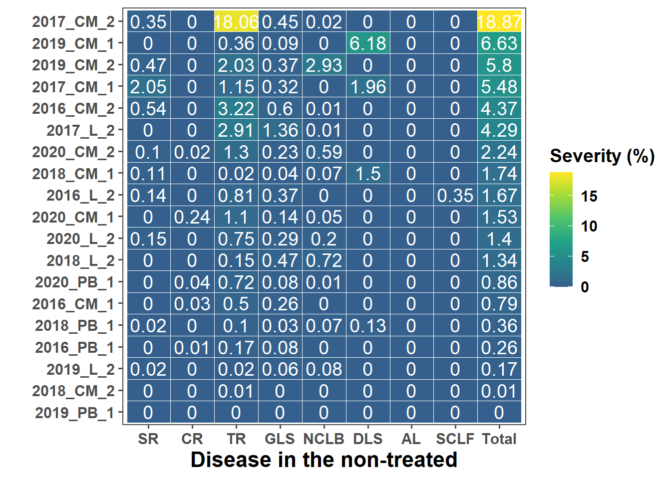

ggsave("fig/heat_disease.png", bg = "white", dpi = 600, height = 8, width = 12)

p_net <- ggplot(econ_tab, aes(x = pressure, y = Net)) +
  geom_hline(yintercept = 0, linewidth = 0.4) +
  geom_col(width = 0.55, fill = "steelblue") +
  geom_errorbar(aes(ymin = Net_lb, ymax = Net_ub), width = 0.1) +
  labs(y = "Net return (R$ ha−1)", x = NULL) +
  theme_half_open()

p_net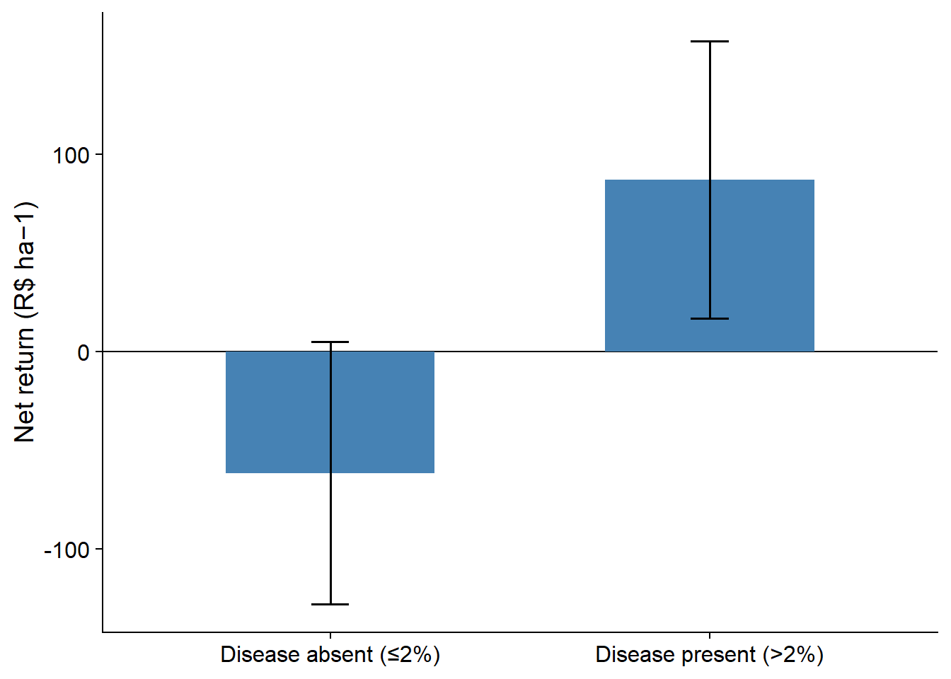

Yield

dados <- gsheet2tbl("https://docs.google.com/spreadsheets/d/1pUGN7bPHtENsO8eb-f8J1q6_pbMqm86bVnaNlgClleo/edit?usp=sharing")

dados2 <- dados |> 
  mutate(trial = interaction(year, location, season, hybrid))

dados3 <- dados2 |> 
  dplyr::group_by(trial, year, location, season, hybrid, technology, application) |>
  dplyr::summarize(sev = mean(severity),
            yld = mean(yield2),
            sd_sev = sd(severity),
            sd_yld = sd(yield2),
            n = n()
            )

dados_meta <- dados3 %>%
  dplyr::select(trial, year, location, season, hybrid, technology, application, yld, sd_yld, n, sev) %>%
  pivot_wider(
    names_from = application,
    values_from = c(yld, sd_yld,n, sev),
    names_sep = "_"
  ) %>%
    dplyr::mutate(
    study_id = paste(trial, year, location, season, hybrid, sep = "_"),
    pressao = ifelse(sev_check > 10, "high", "low"),
    yi = yld_treated - yld_check,
    sei = sqrt((sd_yld_treated^2 / n_treated) + (sd_yld_check^2 / n_check))
  ) %>%
  drop_na(yi, sei) 

dados_meta

library(ggthemes)

metaa = dados_meta %>% 
   filter(sev_check >=5) %>% 
  filter(yld_check <= 12000)

median(metaa$sev_check)

[1] 10.28333

yield_plot = metaa %>% 
  ggplot(aes(yld_check))+
  geom_histogram(color = "white",fill = "black", bins = 10)+
  scale_x_continuous(breaks = c(5000,7500,10000,12500),
                     limits = c(5000, 12500))+
  facet_wrap(~season,labeller = as_labeller(c(
    "first" = "",
    "second" = " "
  )))+
  theme_few()+
  labs(x = "Yield (kg/ha)",
       y = "Frequency")+
  theme(text = element_text(size = 8, face = "bold"),
        axis.text.x = element_text(size = 8, face = "bold", angle = 45, vjust = 0.5),   
        axis.text.y = element_text(size = 8, face = "bold"),
        axis.title = element_text(size = 12, face = "bold"),
        strip.text = element_text(size = 12))
yield_plot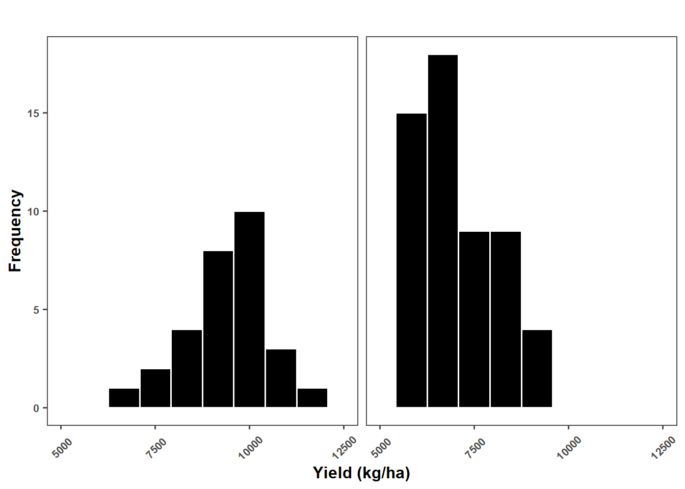

Severity

sev_plot = metaa %>% 
  ggplot(aes(sev_check))+
  geom_histogram(color = "white",fill = "black", bins = 10)+
  facet_wrap(~season,labeller = as_labeller(c(
    "first" = "First",
    "second" = "Second"
  )))+
  theme_few()+
  labs(x = "Severity (%)",
       y = "Frequency")+
  theme(text = element_text(size = 8, face = "bold"),
        axis.text.x = element_text(size = 8, face = "bold", angle = 45, vjust = 0.5),   
        axis.text.y = element_text(size = 8, face = "bold"),
        axis.title = element_text(size = 12, face = "bold"),
        strip.text = element_text(size = 12))

sev_plot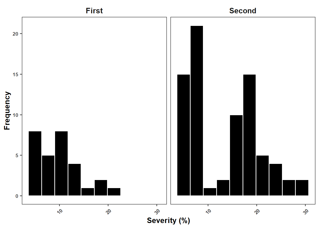

Map

library(dplyr)
library(ggplot2)
library(ggrepel)
library(maps)


# Número de híbridos por location + coordenadas
loc_hybrids <- dados %>%
  group_by(location, season, lat, lon) %>%
  summarise(n_hybrids = n_distinct(hybrid), .groups = "drop")

loc_hybrids$lat = NULL
loc_hybrids$lon = NULL
loc_hybrids$lat = c(-24.09,-24.09,-23.356,-26.1255)
loc_hybrids$lon = c(-52.356389,-52.356389,-51.158889,-52.65)

library(scales)
library(ggspatial) 
library(gsheet)
library(ggrepel)
library(cowplot)
library(rnaturalearth)
library(rnaturalearthdata)
library(sf)
library(tidyverse)

#install.packages("devtools") # I guess you also need this
#devtools::install_github("ropensci/rnaturalearthhires")

BRA = ne_states(
  country = "Brazil",
  returnclass = "sf"
)
library(geobr)
municipios <- read_municipality(code_muni = "all", year = 2020)
municipios = municipios %>% filter(name_state ==  c("Paraná"))

states <- filter(BRA, 
                 name_pt == "Paraná")
unique(BRA$name_pt)

 [1] "Rio Grande do Sul"   "Roraima"             "Pará"               
 [4] "Acre"                "Amapá"               "Mato Grosso do Sul" 
 [7] "Paraná"              "Santa Catarina"      "Amazonas"           
[10] "Rondônia"            "Mato Grosso"         "Maranhão"           
[13] "Piauí"               "Ceará"               "Rio Grande do Norte"
[16] "Paraíba"             "Pernambuco"          "Alagoas"            
[19] "Sergipe"             "Bahia"               "Espírito Santo"     
[22] "Rio de Janeiro"      "São Paulo"           "Goiás"              
[25] "Federal"             "Minas Gerais"        "Tocantins"          

states = states %>% 
  mutate(id = case_when(
    name_pt == "Paraná" ~ "PR"))

SUL = ne_states(
  country = c("Argentina", "Uruguay", "Paraguay", "Colombia", "Bolivia"),
  returnclass = "sf")

br_sf <- ne_states(geounit = "brazil",
                   returnclass = "sf")


library(ggplot2)
library(cowplot)  

library(ggplot2)
library(ggrepel)
library(dplyr)
library(ggthemes)
library(ggspatial)
loc_hybrids <- loc_hybrids[-1, ]
map3 <- loc_hybrids |>
  ggplot() +
  
  # Mapa base do Brasil
  geom_sf(data = BRA, fill = "white", color = "gray60", size = 0.4) +
  
  # Destacar o Paraná
  geom_sf(data = subset(BRA, postal %in% c("PR")), 
          fill = NA, color = "black", size = 1) +
  
  # Siglas dos estados
  geom_text(data = states, aes(x = longitude, y = latitude, label = id), 
            size = 5, hjust = 0.8, color = "black", fontface = "bold") +
  
  # Pontos das localidades
  geom_point(data = loc_hybrids, aes(x = lon, y = lat), 
             alpha = 0.8) +
  
  # Nomes das cidades com linhas
  geom_text_repel(
    data = loc_hybrids,
    aes(x = lon, y = lat, label = location),
    size = 4,
    fontface = "bold",
    color = "black",
    min.segment.length = 0,
    box.padding = 0.3,
    segment.color = "gray30",
    segment.size = 0.4
  ) +
  
  # Tema e ajustes de mapa
  theme_minimal_grid() +
  coord_sf(xlim = c(-58, -45), ylim = c(-27, -22), expand = FALSE) +
  
  # Legenda personalizada
  guides(size = FALSE,  
         color = guide_colorbar(title = "Severity (%)", 
                                direction = "horizontal",
                                title.position = "top")) +
  
  # Estilo da legenda e borda do painel
  theme(
    legend.position = c(0.9, 0.01),  
    legend.justification = c(1, 0),
    legend.direction = "horizontal",
    legend.title.align = 0.5,
    panel.border = element_rect(color = "black", fill = NA, size = 1),
    axis.title = element_text(face = "bold")
  ) +
  
  # Adiciona seta de norte
  annotation_north_arrow(location = "br", which_north = "true", 
                         pad_x = unit(5.86, "in"), pad_y = unit(0.3, "in"), 
                         style = north_arrow_fancy_orienteering, 
                         height = unit(1.2, "cm"), width = unit(1.1, "cm")) +
  
  # Barra de escala
  annotation_scale(location = "br", 
                   width_hint = 0.1, 
                   height = unit(0.2, "cm"), 
                   text_cex = 0.6, 
                   pad_x = unit(5.8, "in"), 
                   pad_y = unit(0.2, "in")) +
  
  # Eixos
  labs(x = "Longitude", y = "Latitude")

map3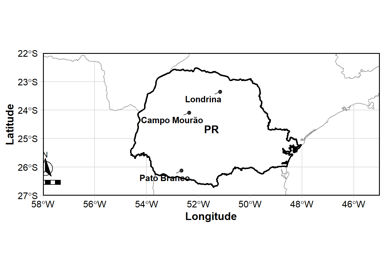

pr_municipios <- read_municipality(code_muni = "all", year = 2020) %>%
  filter(name_state == "Paraná")

BRA <- ne_states(country = "Brazil", returnclass = "sf")
pr_estado <- BRA %>% filter(name_pt == "Paraná")
map2 = loc_hybrids #|> filter(estado == "PR")

mapa_brasil <- ggplot() +
  geom_sf(data = BRA, fill = "white", color = "black", size = 0.2) +  
  geom_sf(data = subset(BRA, postal %in% c("PR")), 
          fill = "gray40", color = "black", size = 0.6) +  
  theme_map() +
    theme(
    panel.background = element_rect(fill = "white", color = NA),  
    plot.background = element_rect(fill = "white", color = NA),   
    panel.border = element_rect(color = "black", fill = NA, size = 1)) 

library(patchwork)
mapp = map3 + 
  inset_element(mapa_brasil, 
                left = 0.8, bottom = 0.5,  
                right = 0.99, top = 0.95) 

library(cowplot)


right_panel <- plot_grid(
  sev_plot, yield_plot,
  ncol = 1,
  labels = c("(b)", "(c)"),
  label_size = 14,
  label_fontface = "bold",
  align = "v"
)


final_plot <- plot_grid(
  mapp, right_panel,
  ncol = 2,
  rel_widths = c(2, 1),     
  labels = c("(a)",""),
  label_size = 14,
  label_fontface = "bold",
  label_x = 0.02,
  label_y = 0.98,
  align = "h"
)

final_plot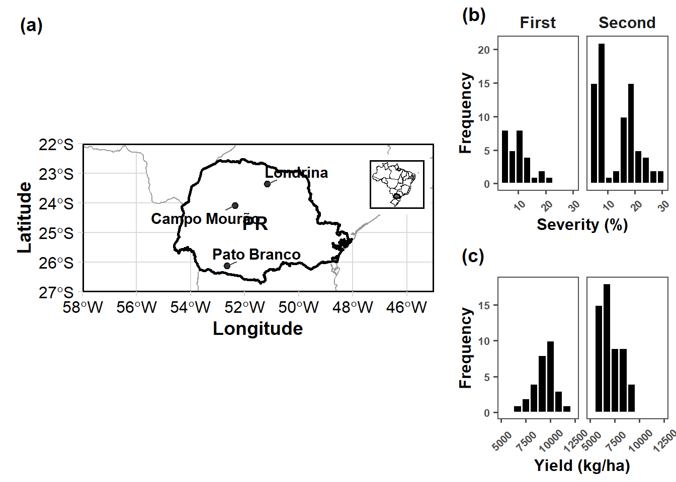

ggsave("fig/map.png", height=4, width=10, dpi = 600, bg = "white")