This chunk initializes the computational environment and defines the core parameters used throughout the analysis. It specifies the maximum lag window, the flexibility of the exposure–lag relationships, and the set of climatic variables to be analyzed. These parameters determine the structure of the Distributed Lag Non‑Linear Model (DLNM) and ensure consistency across all subsequent steps of the workflow.

Packages, options and parameters

  library(dplyr)
  library(tidyr)
  library(readr)
  library(readxl)
  library(dlnm)
  library(brms)
  library(ggplot2)
  library(posterior)
  library(purrr)


set.seed(20251218)

# ------------------------------- Parameters ----------------------------------
END_DAP   <- 85     # 85 (disease assessment, ~R6)
LAG_MAX   <- 85     # maximum lag (days before to END_DAP)
DF_VAR    <- 4      # flexibility in the exposure dimension (ns)
DF_LAG    <- 4      # flexibility in the lag dimension (ns)
SEPARATOR <- LAG_MAX

VARS <- c("tmax","rain_cum","vpd")

LAG_BAND_A <- 0:40
LAG_BAND_B <- 41:LAG_MAX

This section imports the epidemiological dataset and performs initial preprocessing required for DLNM analysis. Disease severity observations are aligned with their corresponding planting dates, and a unique identifier is created for each epidemic. The data are then filtered to retain only complete observations, ensuring consistency between disease assessments and exposure histories.

Data importation and pre organization

ERA5 weather extraction

epi <- readxl::read_xlsx("data/ts_check.xlsx")
epi = epi %>% 
  mutate(
    PD85 = planting_date+85
  )

epi$planting_date = as.Date(epi$planting_date)

epi = epi %>% 
  mutate(
    PD85 = planting_date + 85
  )

epi_use <- epi |>
  rename(
    sev = mean_sev
  ) |>
  filter(!is.na(sev)) |>
  mutate(
    planting_date = as.Date(planting_date, origin = "1899-12-30"),
    epi_id = row_number(),
    siteyear = paste0(location, "_", year)
  )

epi_use

These exploratory summaries describe the distribution of disease severity across years and regions. They provide a preliminary understanding of temporal and spatial variability in the dataset, which is essential for interpreting later modeling results.

epi_use %>% 
  summarise(
    mean = mean(sev),
    sd = sd(sev),
    min = min(sev),
    max = max(sev)
  )

mean_year = epi_use %>% 
  group_by(year) %>% 
  summarise(
    mean = mean(sev),
    min = min(sev),
    max = max(sev),
    sd = sd(sev))

mean_year$year = mean_year$year-1
mean_year

mean_year %>% 
  ggplot(aes(year,mean))+
  geom_line()+
  geom_point()+
  theme_bw()+
  scale_x_continuous(breaks=c(2012,2013,2014,2015,2016,2017,
                              2018,2019,2020,2021,2022,2023,2024), limits = c(2012,2024))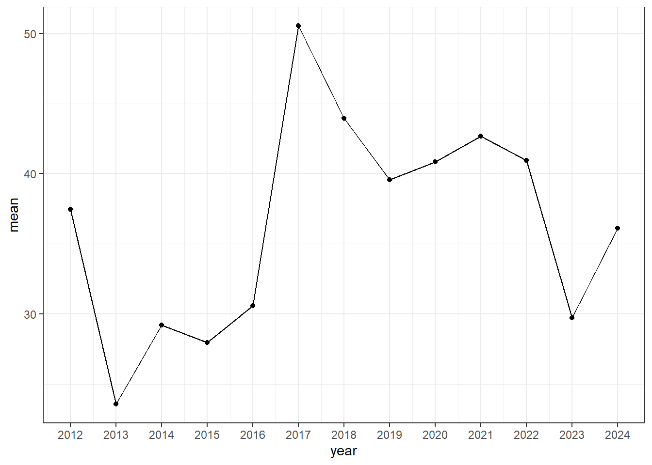

epi_use %>% 
  group_by(state) %>% 
  summarise(
    mean = mean(sev),
    min = min(sev),
    max = max(sev),
    sd = sd(sev)
  )

epi_use %>% 
  group_by(year,state) %>% 
  summarise(
    mean = mean(sev)
  ) %>% 
  ggplot(aes(as.factor(year),mean))+
  geom_bar(stat = "identity")+
  facet_wrap(~state)+
  theme(axis.text.x = element_text(angle = 45))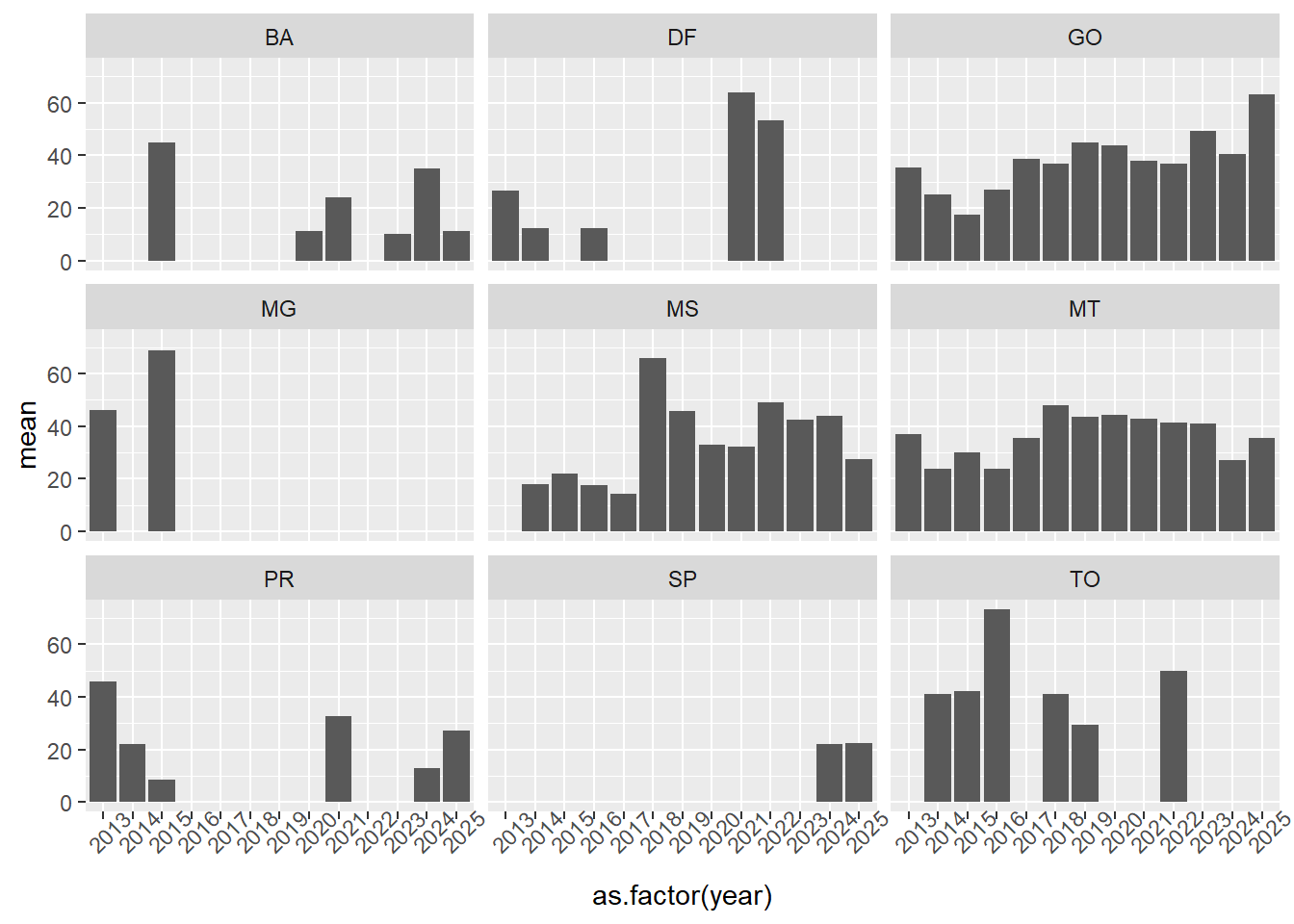

This step links each epidemic to its corresponding daily weather series. Climatic variables are derived and transformed to represent biologically meaningful drivers of disease development, including accumulated precipitation and vapor pressure deficit (VPD). The resulting dataset contains complete exposure histories from planting to disease assessment for each epidemic.

library(r4pde)
wx = get_era5(
  data = epi_use,
  days_around = "85",
  date_col = "planting_date",
  study_col = "epi_id",
  pars = c("temperature_2m", "relative_humidity_2m", "precipitation", "dewpoint_2m"),
  models = NULL,
  direction = "forth"
)


colnames(wx) = c("planting_date", "tmean","tmax","tmin","rh","rain","t2mdew","longitude","latitude","epi_id")


unique(wx$epi_id)

wx_use <- epi_use |>
  select(study,year,location,epi_id,state) %>% 
  left_join(wx, by = "epi_id")

wx_use$dpp <- rep(0:85, times = 254)


es <- function(T) { 0.6108 * exp((17.27 * T) / (T + 237.3)) }
wx_use <- wx_use |>
  mutate(vpd = es(tmean) * (1 - rh / 100))

#wx_use = wx_use %>% 
  #filter(dpp >=15)


wx_use <- wx_use |>
  arrange(epi_id, planting_date) |>
  group_by(epi_id) |>
  mutate(rain_cum = cumsum(rain)) |>
  ungroup()

#writexl::write_xlsx(wx_use,"data/ERA5_weather.xlsx")

wx_use = read_xlsx("data/ERA5_weather.xlsx")

Templates to cross-basis (shared)

This step constructs shared cross-basis templates for each climatic variable using the DLNM framework. Exposure histories from all epidemics are concatenated into a pooled structure with artificial separation gaps to prevent carryover effects across epidemics. These templates define the functional structure used to represent how climatic exposures vary across both intensity and lag time.

# ---- Chunk 2: cross-basis templates ----------------------------------------
build_pooled_series <- function(wx_long, var, sep_n = SEPARATOR) {
  ids <- unique(wx_long$epi_id)
  out <- vector("list", length(ids))
  for (i in seq_along(ids)) {
    v <- wx_long |> filter(epi_id == ids[i]) |> arrange(dpp) |> pull(.data[[var]])
    out[[i]] <- c(v, rep(NA_real_, sep_n))
  }
  unlist(out)
}

cb_templates <- list()
for (v in VARS) {
  stopifnot(v %in% names(wx_use))
  x_pool <- build_pooled_series(wx_use, v, sep_n = SEPARATOR)
  cb_templates[[v]] <- dlnm::crossbasis(
    x_pool, lag = LAG_MAX,
    argvar = list(fun = "ns", df = DF_VAR),
    arglag = list(fun = "ns", df = DF_LAG)
  )
}

Epidemic matrix (design)

Disease severity was observed once per epidemic at the assessment time, whereas climatic exposures were recorded daily over the entire growing period. To reconcile these different temporal resolutions within the DLNM framework, the lagged exposure histories of each epidemic were mapped onto epidemic-level covariates using pre-defined cross-basis templates.

For each climatic variable, the daily exposure series of an epidemic was transformed into a vector of basis coefficients corresponding to the last observed time point (the assessment day). This operation collapses the full distributed lag structure into a single row per epidemic while preserving the cumulative contribution of past exposures encoded by the DLNM. By applying the same cross-basis template to all epidemics, this step ensures that each epidemic is represented within a common functional space, allowing the resulting coefficients to be estimated consistently within a generalized mixed-effects model.

The resulting epidemic-level design matrix contains one row per epidemic and multiple columns per climatic variable, each column corresponding to a specific exposure–lag basis function. These columns serve as fixed-effect predictors in the inferential model, linking past climatic conditions to disease severity through the DLNM representation.

# ---- Chunk 3: per-epidemic design (one row per epidemic) -------------------
extract_last_cb_row <- function(x, cb_template) {
  cb <- dlnm::crossbasis(
    x, lag = LAG_MAX,
    argvar = attr(cb_template, "argvar"),
    arglag = attr(cb_template, "arglag")
  )
  as.numeric(cb[length(x), ])
}

build_design_for_var <- function(wx_long, var, cb_template, prefix) {
  X <- wx_long |>
    group_by(epi_id) |>
    summarise(cb = list(extract_last_cb_row(.data[[var]], cb_template)),
              .groups = "drop")
  p  <- length(X$cb[[1]])
  nm <- paste0(prefix, seq_len(p))
  X  |> mutate(cb = lapply(cb, setNames, nm)) |> tidyr::unnest_wider(cb)
}

X_list <- map(VARS, ~ build_design_for_var(wx_use, .x, cb_templates[[.x]],
                                           prefix = paste0("cb_", .x, "_")))
names(X_list) <- VARS

X <- reduce(X_list, left_join, by = "epi_id")

dat <- epi_use |>
dplyr::select(epi_id, sev, siteyear, year, location, state, latitude, longitude, planting_date, PD85) |>
  left_join(X, by = "epi_id")


#dat <- epi_use |>
#dplyr::select(epi_id, sev, siteyear, year, location, state, lat, longitude, planting_date) |>
#  left_join(X, by = "epi_id")

This step converts the full daily exposure histories into epidemic-level predictors that retain the cumulative and delayed effects of climate encoded by the DLNM. The transformation allows the distributed lag structure to be estimated using a single observation per epidemic while maintaining biological interpretability of the climatic effects across time.

Modeling framework

Inferential framework and model fitting

After constructing epidemic-level DLNM design matrices, disease severity was modeled using a generalized mixed-effects framework. Because the response variable represents a proportion bounded between 0 and 1, a beta regression with a logit link was adopted. This formulation allows flexible modeling of the mean disease severity while respecting the bounded nature of the data.

The DLNM cross-basis coefficients derived for each climatic variable were included as fixed effects in the linear predictor, linking past climatic exposures to disease severity through their distributed and non-linear effects. To account for unobserved heterogeneity among epidemics conducted at different locations and years, a random intercept was specified at the site–year level. This hierarchical structure captures baseline differences in disease pressure that are not explained by the climatic covariates.

Importantly, the DLNM itself does not perform inference; rather, it defines the structure of the predictors. All statistical inference—including estimation of coefficients, uncertainty quantification, and hypothesis testing—is carried out within the mixed-effects beta regression model. Thus, this step represents the point at which the distributed lag non-linear effects are formally estimated and interpreted.

# ---- Chunk 4: fit linear mixed model ------------------------------
cb_terms <- paste(names(dat)[grepl("^cb_", names(dat))], collapse = " + ")
fml <- as.formula(paste0("sev ~ 1 + (1|siteyear) + ", cb_terms))

library(glmmTMB)
dat$sev  = dat$sev/100
  
  
fit_tmb <- glmmTMB( 
  formula = fml,
  data = dat,
  family = beta_family(link = "logit")
)


summary(fit_tmb)

 Family: beta  ( logit )
Formula:          
sev ~ 1 + (1 | siteyear) + cb_tmax_1 + cb_tmax_2 + cb_tmax_3 +  
    cb_tmax_4 + cb_tmax_5 + cb_tmax_6 + cb_tmax_7 + cb_tmax_8 +  
    cb_tmax_9 + cb_tmax_10 + cb_tmax_11 + cb_tmax_12 + cb_tmax_13 +  
    cb_tmax_14 + cb_tmax_15 + cb_tmax_16 + cb_rain_cum_1 + cb_rain_cum_2 +  
    cb_rain_cum_3 + cb_rain_cum_4 + cb_rain_cum_5 + cb_rain_cum_6 +  
    cb_rain_cum_7 + cb_rain_cum_8 + cb_rain_cum_9 + cb_rain_cum_10 +  
    cb_rain_cum_11 + cb_rain_cum_12 + cb_rain_cum_13 + cb_rain_cum_14 +  
    cb_rain_cum_15 + cb_rain_cum_16 + cb_vpd_1 + cb_vpd_2 + cb_vpd_3 +  
    cb_vpd_4 + cb_vpd_5 + cb_vpd_6 + cb_vpd_7 + cb_vpd_8 + cb_vpd_9 +  
    cb_vpd_10 + cb_vpd_11 + cb_vpd_12 + cb_vpd_13 + cb_vpd_14 +  
    cb_vpd_15 + cb_vpd_16
Data: dat

      AIC       BIC    logLik -2*log(L)  df.resid 
   -181.3      -0.9     141.6    -283.3       203 

Random effects:

Conditional model:
 Groups   Name        Variance Std.Dev.
 siteyear (Intercept) 0.1281   0.3579  
Number of obs: 254, groups:  siteyear, 199

Dispersion parameter for beta family (): 13.4 

Conditional model:
                Estimate Std. Error z value Pr(>|z|)   
(Intercept)    -91.43799   33.72773  -2.711  0.00671 **
cb_tmax_1        0.71561    0.55498   1.289  0.19725   
cb_tmax_2        0.43579    0.44981   0.969  0.33263   
cb_tmax_3       -0.32470    0.33756  -0.962  0.33610   
cb_tmax_4       -0.26453    0.50751  -0.521  0.60221   
cb_tmax_5        0.73994    0.37300   1.984  0.04728 * 
cb_tmax_6       -0.02880    0.28873  -0.100  0.92055   
cb_tmax_7       -0.13123    0.22112  -0.594  0.55284   
cb_tmax_8        0.04672    0.29409   0.159  0.87378   
cb_tmax_9        1.38327    1.13884   1.215  0.22451   
cb_tmax_10       0.86710    0.93005   0.932  0.35118   
cb_tmax_11      -0.55799    0.71165  -0.784  0.43299   
cb_tmax_12      -0.17607    1.08801  -0.162  0.87144   
cb_tmax_13       0.10668    0.47650   0.224  0.82284   
cb_tmax_14       0.31631    0.35730   0.885  0.37601   
cb_tmax_15      -0.51349    0.41931  -1.225  0.22072   
cb_tmax_16       0.05704    0.40368   0.141  0.88764   
cb_rain_cum_1   -2.19667    0.72998  -3.009  0.00262 **
cb_rain_cum_2   -1.42815    0.64735  -2.206  0.02737 * 
cb_rain_cum_3    5.09056    2.08157   2.446  0.01446 * 
cb_rain_cum_4   -3.42281    1.42454  -2.403  0.01627 * 
cb_rain_cum_5   -1.28407    0.47389  -2.710  0.00674 **
cb_rain_cum_6   -1.17585    0.50781  -2.316  0.02058 * 
cb_rain_cum_7    4.59117    1.68803   2.720  0.00653 **
cb_rain_cum_8    0.26333    1.76334   0.149  0.88129   
cb_rain_cum_9   -4.05763    1.48428  -2.734  0.00626 **
cb_rain_cum_10  -2.20038    1.90819  -1.153  0.24886   
cb_rain_cum_11 -17.85349   22.99215  -0.776  0.43745   
cb_rain_cum_12 -47.39872   34.94649  -1.356  0.17500   
cb_rain_cum_13  -0.68314    0.78249  -0.873  0.38264   
cb_rain_cum_14   0.03376    2.86137   0.012  0.99059   
cb_rain_cum_15 -48.31432   42.32921  -1.141  0.25371   
cb_rain_cum_16 -78.54418   64.56302  -1.217  0.22378   
cb_vpd_1        -0.15554    0.21531  -0.722  0.47006   
cb_vpd_2         0.13762    0.20542   0.670  0.50289   
cb_vpd_3         0.28504    0.14482   1.968  0.04905 * 
cb_vpd_4         0.14017    0.24275   0.577  0.56365   
cb_vpd_5        -0.23928    0.21029  -1.138  0.25519   
cb_vpd_6         0.31839    0.17996   1.769  0.07686 . 
cb_vpd_7        -0.14754    0.17915  -0.824  0.41018   
cb_vpd_8         0.01735    0.21960   0.079  0.93702   
cb_vpd_9        -0.42078    0.48967  -0.859  0.39017   
cb_vpd_10        0.09286    0.45933   0.202  0.83979   
cb_vpd_11        1.45724    0.49684   2.933  0.00336 **
cb_vpd_12       -0.46291    0.57102  -0.811  0.41755   
cb_vpd_13       -0.25608    0.57263  -0.447  0.65473   
cb_vpd_14       -0.70089    0.41145  -1.704  0.08848 . 
cb_vpd_15        2.27111    0.88535   2.565  0.01031 * 
cb_vpd_16       -1.09237    0.66406  -1.645  0.09997 . 
---
Signif. codes:  0 '***' 0.001 '**' 0.01 '*' 0.05 '.' 0.1 ' ' 1

This modeling step represents the inferential core of the analysis. The DLNM defines how climatic effects are structured across exposure levels and time lags, while the mixed-effects beta regression estimates the magnitude, direction, and uncertainty of these effects. The resulting model quantifies how past climatic conditions jointly shape disease severity at the assessment time, accounting for both delayed responses and unobserved heterogeneity among site–year combinations.

Model performance

After fitting the DLNM-based mixed-effects beta regression model, fitted values were obtained for each epidemic to quantify the model-implied mean disease severity at the assessment time. These fitted values represent the expected severity conditional on the estimated distributed lag non-linear effects of climatic variables and the random site–year effects.

Predictions were generated on the response scale, yielding values directly interpretable as mean disease severity proportions. By attaching these fitted values to the epidemic-level dataset, this step facilitates subsequent model evaluation, diagnostic checks, and graphical comparison between observed and model-implied disease severity. Importantly, these predictions are not used to refit the model; rather, they summarize how the inferred DLNM structure translates into expected epidemiological outcomes for the observed data.

t = predict(fit_tmb, newdata = dat, type = "response")


dat2 = dat
dat2$t = t

This step translates the inferred DLNM effects into epidemic-level expectations of disease severity on the natural response scale. The fitted values summarize how the combined, lagged influence of climate and site–year heterogeneity manifests in expected disease outcomes, providing a direct link between the statistical model and epidemiological interpretation.

Agreement between observed and model-implied severity (CCC decomposition)

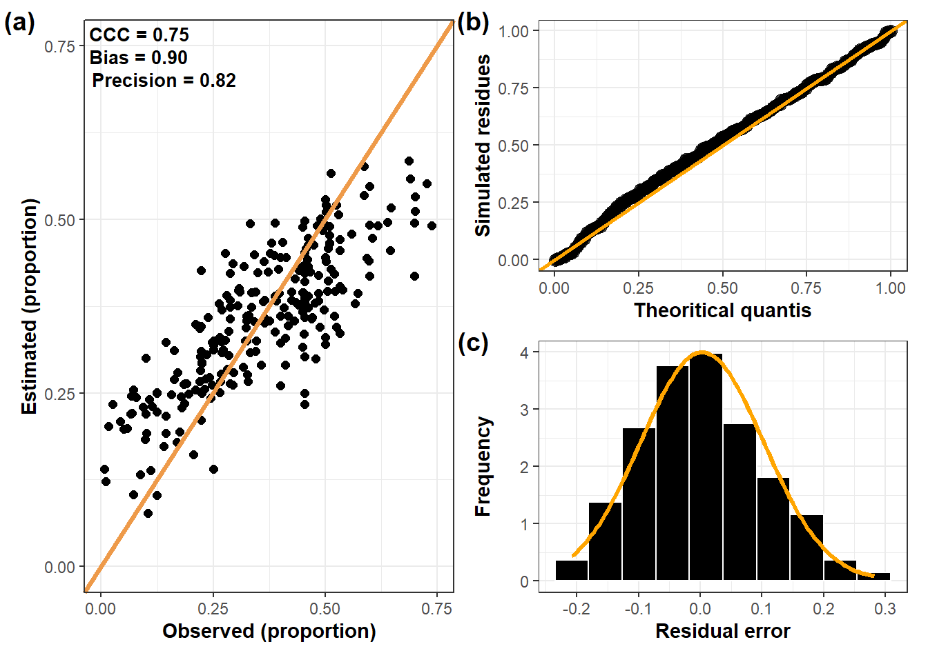
To quantify how well the fitted model reproduces observed disease severity on the response scale, we evaluated agreement between observed severities (\(y_i\)) and fitted mean severities (\(\hat{\mu}_i\)) using Lin’s Concordance Correlation Coefficient (CCC). CCC measures both (i) precision (how tightly predictions follow the observed variability) and (ii) accuracy/bias (how close predictions are to the 1:1 line). This provides a single interpretable agreement metric that complements visual diagnostics.

We also report the two standard CCC components: the Pearson correlation (precision component) and the bias correction factor (accuracy component). Together, these summarize whether lack of agreement is driven primarily by random dispersion (low precision), systematic bias (low accuracy), or both.

library(epiR)

tt = epi.ccc(dat2$sev,dat2$t)

tt$rho.c

tt$C.b

[1] 0.9089234

r <- tt$rho.c[,1]/tt$C.b
r

[1] 0.8288625

gc()

          used  (Mb) gc trigger  (Mb) max used  (Mb)
Ncells 3724727 199.0    5883457 314.3  5883457 314.3
Vcells 9180000  70.1   26948174 205.6 26948174 205.6

Graphical calibration and residual error distribution

To complement the CCC summary, we visualized model calibration by plotting observed severity (\(y_i\)) against fitted mean severity (\(\hat{\mu}_i\)) with a 1:1 reference line. Points close to this line indicate good calibration; systematic deviations reflect bias (e.g., underprediction at high severities).

We additionally computed residual errors on the response scale and examined their empirical distribution via a histogram, overlaying a normal density with matching mean and standard deviation. While the beta regression model does not assume normal residuals on the response scale, this visualization provides a simple check for gross asymmetry, heavy tails, or systematic shifts (non-zero mean error) that may indicate calibration issues.

CCC  <- 0.75
Bias <- 0.90
Precision <- 0.82

library(scales)
lab <- paste0(
  "CCC = ", number(CCC, accuracy = 0.01, decimal.mark = "."),
  "\nBias = ", number(Bias, accuracy = 0.01, decimal.mark = "."),
  "\nPrecision = ", number(Precision, accuracy = 0.01, decimal.mark = ".")
)


model = dat2 %>% 
  ggplot(aes(sev,t))+
  geom_jitter(size = 2)+
  #geom_smooth(method = "lm", se = F, color = "orange")+
   geom_abline(slope = 1, intercept = 0, color = "tan2",
              linetype = "solid", size = 1.4) +
  scale_x_continuous(breaks=c(0.00, 0.25, 0.50,0.75), limits = c(0,0.75))+
  scale_y_continuous(breaks=c(0.00, 0.25, 0.50,0.75), limits = c(0,0.75))+
  theme_bw()+
  coord_cartesian(clip = "off")+
  labs(x = "Observed (proportion)",
       y = "Estimated (proportion)")+
  annotate(
    "text",
    x = -Inf, y = Inf,
    label = lab,
    hjust = -0.05,   
    vjust = 1.1,     
    size = 3.5,
    fontface = "bold",
    lineheight = 1.05
  )+
  theme(axis.title = element_text(face = "bold"))


dat2 = dat2 %>% 
  mutate(
    error = sev - t
  )

mean_res = mean(dat2$error)
sd_res = sd(dat2$error)



hist = dat2 %>% 
  ggplot(aes(error))+
  geom_histogram(aes(y = ..density..), fill = "black", color = "white", bins = 10) + 
  stat_function(fun = dnorm, args = list(mean = mean_res, sd = sd_res), 
                color = "orange", size = 1.2, linetype = "solid")+
  theme_bw()+
 labs(
    x = "Residual error",
    y = "Frequency"
  )+
  theme(axis.title = element_text(face = "bold"))

Simulation-based residual diagnostics (DHARMa)

Because beta mixed models can exhibit complex residual behavior—particularly under non-Gaussian likelihoods and random effects—we evaluated model adequacy using simulation-based residual diagnostics implemented in DHARMa. DHARMa simulates response replicates from the fitted model (including the specified distribution and random effects structure) and constructs scaled residuals that should be approximately Uniform(0,1) under correct model specification.

We then assessed the uniformity of the simulated residuals using a quantile–quantile (QQ) comparison between observed residual quantiles and their theoretical Uniform(0,1) quantiles. Systematic departures from the 1:1 line indicate potential misspecification, such as incorrect distributional assumptions, unmodeled structure, or dispersion issues.

library(DHARMa)
library(ggplot2)

res <- simulateResiduals(fit_tmb)


u <- sort(res$scaledResiduals)
n <- length(u)


theoretical <- ((1:n) - 0.5) / n


df <- data.frame(
  theoretical = theoretical,
  observed = u
)


qq_plot = ggplot(df, aes(x = theoretical, y = observed)) +
  geom_jitter(color = "black", alpha = 0.7, size = 3) +
  geom_abline(slope = 1, intercept = 0, color = "orange", linewidth = 1) +
  labs(
    x = "Theoritical quantis",
    y = "Simulated residues"
  )+
  theme_bw()+
  theme(axis.title = element_text(face = "bold"))

library(patchwork)

(model|qq_plot/hist)+
  plot_annotation(
    tag_levels = "a",
    tag_prefix = "(",
    tag_suffix = ")"
  ) &
  theme(
    plot.tag = element_text(face = "bold", size = 14),
    plot.tag.position = c(0, 1) 
  )

ggsave("fig/model2.png", dpi = 600, width = 8, height = 6)

Cumulative effects

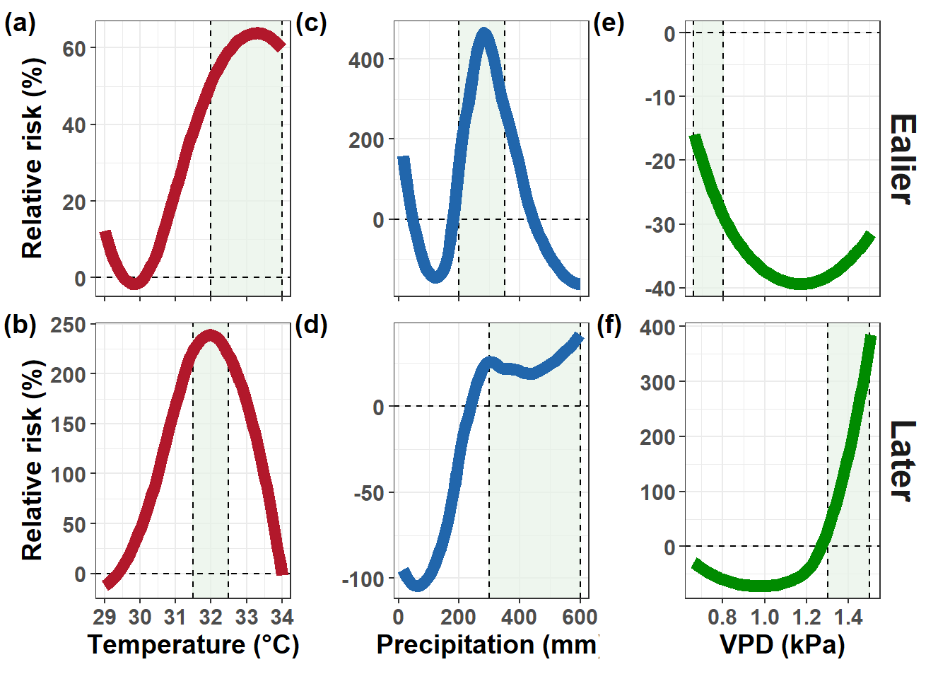
To summarize the distributed effects of climatic variables in an epidemiologically interpretable manner, relative risks were derived from the fitted DLNM by aggregating lag-specific contributions over predefined temporal periods. Rather than interpreting individual lag effects, which may be difficult to relate directly to biological processes, cumulative effects were computed for early and late lag periods corresponding to distinct phases of epidemic development.

For each climatic variable, the DLNM provides an estimated exposure–lag response surface describing how past exposures contribute to disease severity at the assessment time. By summing the lag-specific contributions across a given lag period and exponentiating the resulting linear predictor, a cumulative relative risk is obtained. This quantity represents the proportional change in expected disease severity associated with a given exposure level, relative to a reference value, accounting for the entire exposure history within the specified lag interval.

Lag periods were defined a priori to reflect biologically meaningful phases of the epidemic. The early period (0–40 days before assessment) captures processes related to infection establishment, latent development, and early lesion formation, whereas the late period (41–70 days) reflects symptom expansion and disease expression near the assessment stage. This aggregation facilitates direct comparison of climatic effects across variables and epidemic phases, while preserving the non-linear and delayed structure estimated by the DLNM.

Temperature

Later period (0-40)

var <- "tmax"
cb  <- cb_templates[[var]]

cf  <- coef(summary(fit_tmb))$cond[,1]
vc  <- vcov(fit_tmb)$cond

prefix <- paste0("cb_", var, "_")
idx <- grepl(prefix, names(cf))

beta   <- cf[idx]
vc_sub <- vc[idx, idx]

# values for the complete curve
x_all   <- wx_use[[var]]
grid    <- sort(unique(as.numeric(quantile(x_all, seq(0.05,0.95,by=0.01)))))

# reference (P50) used as centering
P50 <- quantile(x_all, 0.50, na.rm=TRUE)

cp <- crosspred(
  cb,
  coef = beta,
  vcov = vc_sub,
  at   = grid,
  cen  = P50,
  bylag = 1
)

mf <- cp$matfit     # matrix: rows = grid, cols = lags

lag_idx <- suppressWarnings(as.integer(gsub("lag","", colnames(mf))))
if(anyNA(lag_idx)) lag_idx <- 0:(ncol(mf)-1)

colsA <- which(lag_idx %in% 0:40)

# cumulative effect for EACH grid temperature
etaA <- apply(mf[, colsA, drop=FALSE], 1, sum)

RR <- exp(etaA)

rr_sum_t_la <- data.frame(
  tmean = grid,
  RR_med = RR) %>% 
  mutate(
    PERC = (RR_med-1)*100
  )

tmean_RR_second =rr_sum_t_la %>% 
  filter(tmean >=29) %>% 
 #filter(tmean >=5) %>% 
 #filter(tmean >=0.66) %>%
ggplot(aes(x=tmean, y=PERC)) +
  #annotate("rect", xmin = 25, xmax = 26, ymin = -Inf, ymax = Inf,
   #        fill = "lightgreen", color = "lightgreen",alpha = .7) +
  annotate("rect", xmin = 31.5, xmax = 32.5, ymin = -Inf, ymax = Inf, fill = "#E6F2E6", color = "#E6F2E6",alpha = .7) +
  geom_hline(yintercept = 0, linetype=2) +
  geom_vline(xintercept = 31.5, linetype=2) +
  geom_vline(xintercept = 32.5, linetype=2) +
  geom_smooth(size = 3, colour = "#B2182B", se = F) +
  labs(x="Temperature (°C)",
       y="Relative risk (%)") +
  theme_bw()+
  theme(
    text = element_text(face = "bold", size = 14) )

tmean_RR_second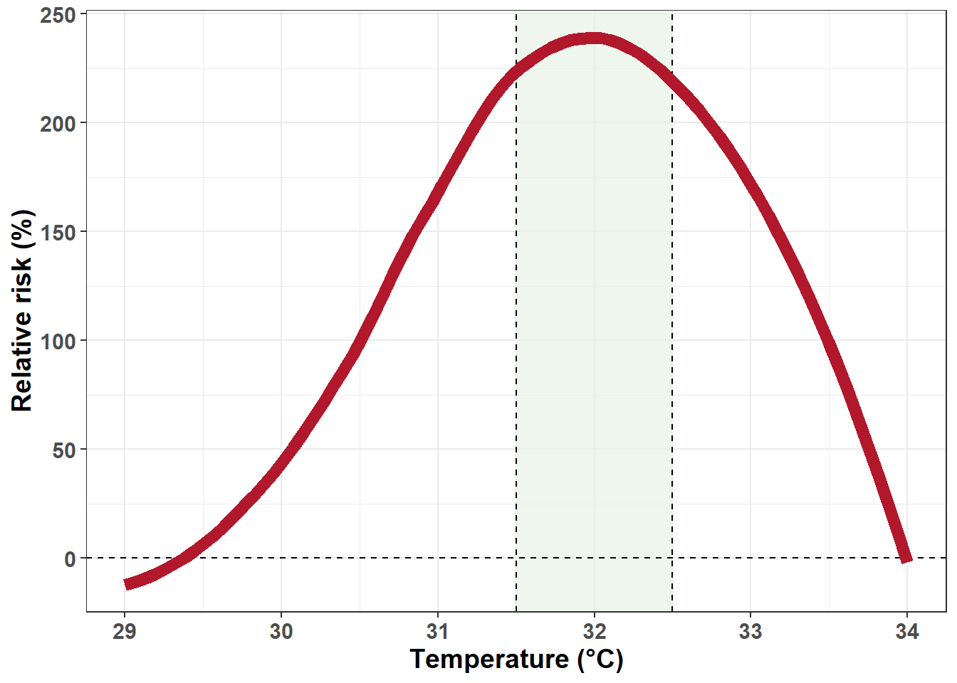

Ealier period (41-85)

var <- "tmax"
cb  <- cb_templates[[var]]

cf  <- coef(summary(fit_tmb))$cond[,1]
vc  <- vcov(fit_tmb)$cond

prefix <- paste0("cb_", var, "_")
idx <- grepl(prefix, names(cf))

beta   <- cf[idx]
vc_sub <- vc[idx, idx]

# values for the complete curve
x_all   <- wx_use[[var]]
grid    <- sort(unique(as.numeric(quantile(x_all, seq(0.05,0.95,by=0.01)))))

# reference (P50) used as centering
P50 <- quantile(x_all, 0.50, na.rm=TRUE)

cp <- crosspred(
  cb,
  coef = beta,
  vcov = vc_sub,
  at   = grid,
  cen  = P50,
  bylag = 1
)

mf <- cp$matfit     # matrix: rows = grid, cols = lags

lag_idx <- suppressWarnings(as.integer(gsub("lag","", colnames(mf))))
if(anyNA(lag_idx)) lag_idx <- 0:(ncol(mf)-1)

colsA <- which(lag_idx %in% 41:85)

# cumulative effect for EACH grid temperature
etaA <- apply(mf[, colsA, drop=FALSE], 1, sum)

RR <- exp(etaA)

rr_sum_t_ea <- data.frame(
  tmean = grid,
  RR_med = RR) %>% 
  mutate(
    PERC = (RR_med-1)*100
  )

tmean_RR_first = rr_sum_t_ea %>% 
  filter(tmean >=29) %>% 
 #filter(tmean >=5) %>% 
 #filter(tmean >=0.66) %>%
ggplot(aes(x=tmean, y=PERC)) +
 #annotate("rect", xmin = 25, xmax = 26, ymin = -Inf, ymax = Inf,
   #        fill = "lightgreen", color = "lightgreen",alpha = .7) +
  annotate("rect", xmin = 32, xmax = 34, ymin = -Inf, ymax = Inf, fill = "#E6F2E6", color = "#E6F2E6",alpha = .7) +
  geom_hline(yintercept = 0, linetype=2) +
  geom_vline(xintercept = 32, linetype=2) +
  geom_vline(xintercept = 34, linetype=2) +
  geom_smooth(size = 3, colour = "#B2182B", se  = F) +
  labs(x="Temperature (°C)",
       y="Relative risk (%)") +
  theme_bw()+
  theme(
    text = element_text(face = "bold", size = 14),
    axis.title.x = element_blank(),
    axis.text.x = element_blank())

    
tmean_RR_first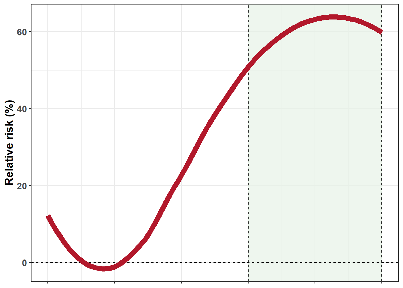

Precipitation

Later period (0-40)

var <- "rain_cum"
cb  <- cb_templates[[var]]

cf  <- coef(summary(fit_tmb))$cond[,1]
vc  <- vcov(fit_tmb)$cond

prefix <- paste0("cb_", var, "_")
idx <- grepl(prefix, names(cf))

beta   <- cf[idx]
vc_sub <- vc[idx, idx]

# values for the complete curve
x_all   <- wx_use[[var]]
grid    <- sort(unique(as.numeric(quantile(x_all, seq(0.05,0.95,by=0.01)))))

# reference (P50) used as centering
P50 <- quantile(x_all, 0.50, na.rm=TRUE)

cp <- crosspred(
  cb,
  coef = beta,
  vcov = vc_sub,
  at   = grid,
  cen  = P50,
  bylag = 1
)

mf <- cp$matfit     # matrix: rows = grid, cols = lags

lag_idx <- suppressWarnings(as.integer(gsub("lag","", colnames(mf))))
if(anyNA(lag_idx)) lag_idx <- 0:(ncol(mf)-1)

colsA <- which(lag_idx %in% 0:40)

# cumulative effect for EACH grid temperature
etaA <- apply(mf[, colsA, drop=FALSE], 1, sum)

RR <- exp(etaA)

rr_sum_r_la <- data.frame(
  tmean = grid,
  RR_med = RR) %>% 
  mutate(
    PERC = (RR_med-1)*100
  )

rain_RR_second =rr_sum_r_la %>% 
  #filter(tmean >=25) %>% 
 filter(tmean >=5) %>% 
 #filter(tmean >=0.66) %>%
ggplot(aes(x=tmean, y=PERC)) +
 #annotate("rect", xmin = 5, xmax = 10, ymin = -Inf, ymax = Inf,
  #         fill = "lightgreen", color = "lightgreen",alpha = .7) +
  annotate("rect", xmin = 300, xmax = 600, ymin = -Inf, ymax = Inf, fill = "#E6F2E6", color = "#E6F2E6",alpha = .7) +
  geom_hline(yintercept = 0, linetype=2) +
  geom_vline(xintercept = 300, linetype=2) +
  geom_vline(xintercept = 600, linetype=2) +
  geom_smooth(size = 3, colour = "#2166AC", se = F) +
  labs(x="Precipitation (mm)",
       y="") +
  theme_bw()+
  theme(
    text = element_text(face = "bold", size = 14) )

rain_RR_second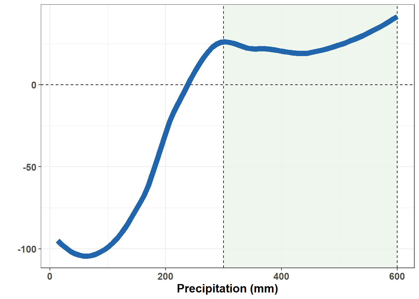

Ealier period (41-85)

var <- "rain_cum"
cb  <- cb_templates[[var]]

cf  <- coef(summary(fit_tmb))$cond[,1]
vc  <- vcov(fit_tmb)$cond

prefix <- paste0("cb_", var, "_")
idx <- grepl(prefix, names(cf))

beta   <- cf[idx]
vc_sub <- vc[idx, idx]

# values for the complete curve
x_all   <- wx_use[[var]]
grid    <- sort(unique(as.numeric(quantile(x_all, seq(0.05,0.95,by=0.01)))))

# reference (P50) used as centering
P50 <- quantile(x_all, 0.50, na.rm=TRUE)

cp <- crosspred(
  cb,
  coef = beta,
  vcov = vc_sub,
  at   = grid,
  cen  = P50,
  bylag = 1
)

mf <- cp$matfit     # matrix: rows = grid, cols = lags

lag_idx <- suppressWarnings(as.integer(gsub("lag","", colnames(mf))))
if(anyNA(lag_idx)) lag_idx <- 0:(ncol(mf)-1)

colsA <- which(lag_idx %in% 41:85)

# cumulative effect for EACH grid temperature
etaA <- apply(mf[, colsA, drop=FALSE], 1, sum)

RR <- exp(etaA)

rr_sum_r_ea <- data.frame(
  tmean = grid,
  RR_med = RR) %>% 
  mutate(
    PERC = (RR_med-1)*100
  )

rain_RR_first = rr_sum_r_ea %>% 
  #filter(tmean >=25) %>% 
 dplyr::filter(tmean >=5) %>% 
 #filter(tmean >=0.66) %>%
ggplot(aes(x=tmean, y=PERC)) +
  ##annotate("rect", xmin = 5, xmax = 10, ymin = -Inf, ymax = Inf,
    #       fill = "lightgreen", color = "lightgreen",alpha = .7) +
   annotate("rect", xmin = 200, xmax = 350, ymin = -Inf, ymax = Inf, fill = "#E6F2E6", color = "#E6F2E6",alpha = .7) +
  geom_hline(yintercept = 0, linetype=2) +
  geom_vline(xintercept = 200, linetype=2) +
  geom_vline(xintercept = 350, linetype=2) +
  geom_smooth(size = 3, colour = "#2166AC", se = F) +
  labs(x="Precipitation (mm)",
       y="") +
  theme_bw()+
  theme(
    text = element_text(face = "bold", size = 14),
    axis.title.x = element_blank(),
    axis.text.x = element_blank())

rain_RR_first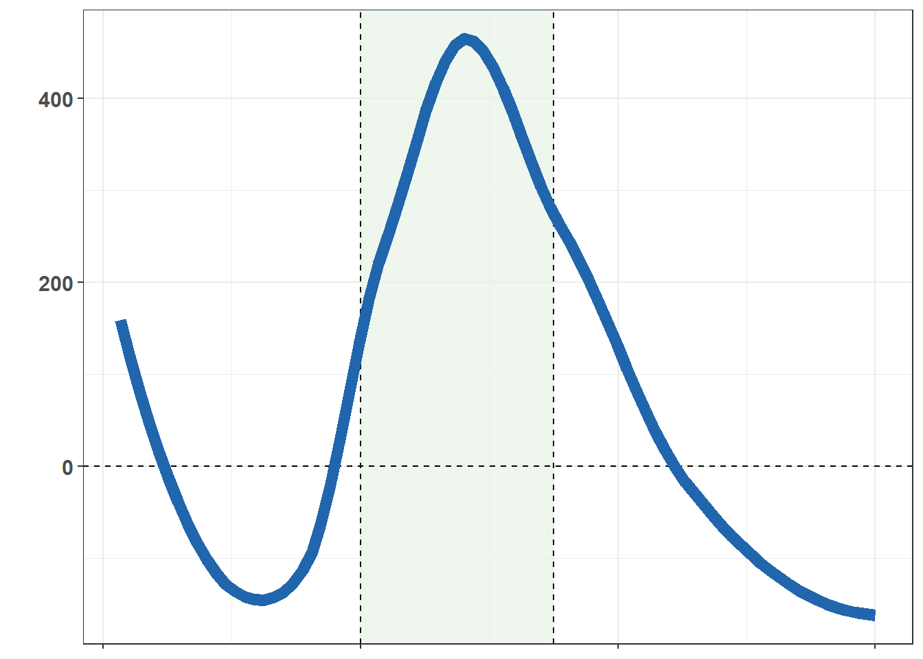

VPD

Later period (0-40)

var <- "vpd"
cb  <- cb_templates[[var]]

cf  <- coef(summary(fit_tmb))$cond[,1]
vc  <- vcov(fit_tmb)$cond

prefix <- paste0("cb_", var, "_")
idx <- grepl(prefix, names(cf))

beta   <- cf[idx]
vc_sub <- vc[idx, idx]

# values for the complete curve
x_all   <- wx_use[[var]]
grid    <- sort(unique(as.numeric(quantile(x_all, seq(0.05,0.95,by=0.01)))))

# reference (P50) used as centering
P50 <- quantile(x_all, 0.50, na.rm=TRUE)

cp <- crosspred(
  cb,
  coef = beta,
  vcov = vc_sub,
  at   = grid,
  cen  = P50,
  bylag = 1
)

mf <- cp$matfit     # matrix: rows = grid, cols = lags

lag_idx <- suppressWarnings(as.integer(gsub("lag","", colnames(mf))))
if(anyNA(lag_idx)) lag_idx <- 0:(ncol(mf)-1)

colsA <- which(lag_idx %in% 0:40)

# cumulative effect for EACH grid temperature
etaA <- apply(mf[, colsA, drop=FALSE], 1, sum)

RR <- exp(etaA)

rr_sum_v_la <- data.frame(
  tmean = grid,
  RR_med = RR) %>% 
  mutate(
    PERC = (RR_med-1)*100
  )

rr_sum_v_la$phase = "Later"

vpd_RR_second =rr_sum_v_la %>% 
  #filter(tmean >=25) %>% 
 #filter(tmean >=5) %>% 
 filter(tmean >=0.66) %>%
 # filter(tmean >=81) %>%
ggplot(aes(x=tmean, y=PERC)) +
##annotate("rect", xmin = 0.66, xmax = 1, ymin = -Inf, ymax = Inf,
  ##         fill = "lightgreen", color = "lightgreen",alpha = .7) +
   annotate("rect", xmin = 1.3, xmax = 1.5, ymin = -Inf, ymax = Inf, fill = "#E6F2E6", color = "#E6F2E6",alpha = .7) +
  geom_hline(yintercept = 0, linetype=2) +
  geom_vline(xintercept = 1.3, linetype=2) +
  geom_vline(xintercept = 1.5, linetype=2) +
  geom_smooth(size = 3, colour = "green4", se = F) +
  labs(x="VPD (kPa)",
       y="") +
  facet_wrap(~phase, strip.position = "right")+
  theme_bw()+
  theme(
    text = element_text(face = "bold", size = 14),
    strip.background = element_blank(),
    strip.text = element_text(size = 18, face = "bold"))

vpd_RR_second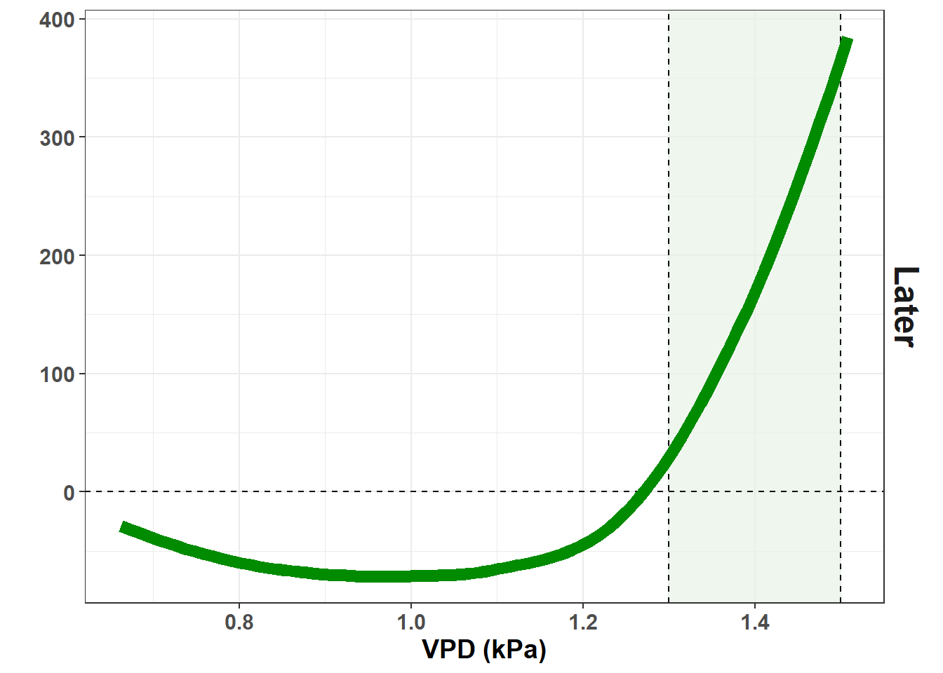

Ealier period (41-85)

var <- "vpd"
cb  <- cb_templates[[var]]

cf  <- coef(summary(fit_tmb))$cond[,1]
vc  <- vcov(fit_tmb)$cond

prefix <- paste0("cb_", var, "_")
idx <- grepl(prefix, names(cf))

beta   <- cf[idx]
vc_sub <- vc[idx, idx]

# values for the complete curve
x_all   <- wx_use[[var]]
grid    <- sort(unique(as.numeric(quantile(x_all, seq(0.05,0.95,by=0.01)))))

# reference (P50) used as centering
P50 <- quantile(x_all, 0.50, na.rm=TRUE)

cp <- crosspred(
  cb,
  coef = beta,
  vcov = vc_sub,
  at   = grid,
  cen  = P50,
  bylag = 1
)

mf <- cp$matfit     # matrix: rows = grid, cols = lags

lag_idx <- suppressWarnings(as.integer(gsub("lag","", colnames(mf))))
if(anyNA(lag_idx)) lag_idx <- 0:(ncol(mf)-1)

colsA <- which(lag_idx %in% 41:85)

# cumulative effect for EACH grid temperature
etaA <- apply(mf[, colsA, drop=FALSE], 1, sum)

RR <- exp(etaA)

rr_sum_v_ea <- data.frame(
  tmean = grid,
  RR_med = RR) %>% 
  mutate(
    PERC = (RR_med-1)*100
  )

rr_sum_v_ea$phase = "Ealier"


vpd_RR_first = rr_sum_v_ea %>% 
 # filter(tmean >=25) %>% 
 #filter(tmean >=5) %>% 
 filter(tmean >=0.66) %>%
ggplot(aes(x=tmean, y=PERC)) +
##annotate("rect", xmin = 0.66, xmax = 1, ymin = -Inf, ymax = Inf,
  #         fill = "lightgreen", color = "lightgreen", alpha = .7) +
  annotate("rect", xmin = 0.66, xmax = 0.80, ymin = -Inf, ymax = Inf, fill = "#E6F2E6", color = "#E6F2E6",alpha = .7) +
  geom_hline(yintercept = 0, linetype=2) +
  geom_vline(xintercept = 0.66, linetype=2) +
  geom_vline(xintercept = 0.80, linetype=2) +
  geom_smooth(size = 3, colour = "green4", se = F) +
  labs(x="Precipitation (mm)",
       y="") +
    facet_wrap(~phase, strip.position = "right")+
  theme_bw()+
  theme(
    text = element_text(face = "bold", size = 14),
    axis.title.x = element_blank(),
    axis.text.x = element_blank(),
    strip.background = element_blank(),
    strip.text = element_text(size = 18, face = "bold"))

vpd_RR_first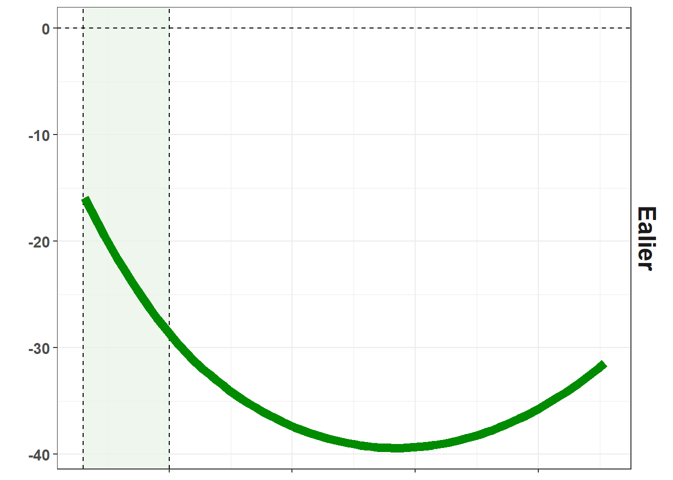

library(patchwork)

(tmean_RR_first/tmean_RR_second|rain_RR_first/rain_RR_second|vpd_RR_first/vpd_RR_second)+
  plot_annotation(
    tag_levels = "a",
    tag_prefix = "(",
    tag_suffix = ")"
  ) &
  theme(
    plot.tag = element_text(face = "bold", size = 14),
    plot.tag.position = c(0, 1) 
  )

#ggsave("fig/RR.png", dpi = 600, width = 12, height = 6)

Daily effect

Temperature

library(dlnm)
library(dplyr)
library(ggplot2)
library(tidyr)

# ==============================================================
# 1) EXTRACT COEFFICIENTS
# ==============================================================

var <- "tmax"
cb  <- cb_templates[[var]]

cf  <- coef(summary(fit_tmb))$cond[,1]
vc  <- vcov(fit_tmb)$cond

idx     <- grepl("^cb_tmax_", names(cf))
beta    <- cf[idx]
vc_sub  <- vc[idx, idx]

stopifnot(length(beta) == ncol(cb))
stopifnot(nrow(vc_sub) == ncol(cb))

# ==============================================================
# 2) DEFINE GRID AND TMEAN RANGE FOR THE HEATMAP
# ==============================================================

x_all <- wx_use[[var]]
P50   <- quantile(x_all, 0.50, na.rm = TRUE)

# Grid used by DLNM
grid <- sort(unique(as.numeric(quantile(
  x_all, seq(0.05, 0.95, by = 0.01), na.rm = TRUE
))))

# Desired values for the heatmap (29 to 34 °C)
#at_vals <- seq(1, 2, length.out = 10000)
at_vals <- seq(29, 34, length.out = 10000)

# Adjust to the REAL grid range (avoids extrapolation)
at_vals <- at_vals[at_vals >= min(grid) & at_vals <= max(grid)]

# ==============================================================
# 3) crosspred IN ALL at-vals (mobile lag)
# ==============================================================

cp <- crosspred(
  cb,
  coef  = beta,
  vcov  = vc_sub,
  at    = at_vals,
  cen   = P50,
  bylag = 1
)

# matrix: rows = tmean values; columns = lags
mf <- cp$matfit

# create lag vectors
lag_idx <- suppressWarnings(as.integer(gsub("lag","",colnames(mf))))
if (anyNA(lag_idx)) lag_idx <- 0:(ncol(mf)-1)

# ==============================================================
# 4) Convert to RR (lag) and then % (% change)
# ==============================================================

RR_mat   <- exp(mf)
PERC_mat <- (RR_mat - 1) * 100

# pivot to tidy format
df_heat <- as.data.frame(PERC_mat)
colnames(df_heat) <- paste0("lag_", lag_idx)
df_heat <- df_heat %>%
  mutate(tmean_val = at_vals) %>%
  pivot_longer(cols = starts_with("lag_"),
               names_to = "lag",
               values_to = "PERC") %>%
  mutate(lag = as.integer(gsub("lag_", "", lag)))

freq_tmax = df_heat %>% 
  ggplot(aes(PERC))+
  geom_histogram(bins = 12, color = "white", fill = "#B2182B")+
  theme_bw(base_size = 12) +
    theme(
    panel.grid = element_blank(),
    axis.title = element_text(face = "bold", size = 12),
    axis.text  = element_text(size = 10),
    legend.title = element_text(face = "bold"),
    plot.title = element_text(face = "bold", size = 13),
    plot.subtitle = element_text(size = 10),
    legend.position = "top"
  )+
  labs(
    x = "Relative risk (RR)",
    y = "Frequency"
  )

freq_tmax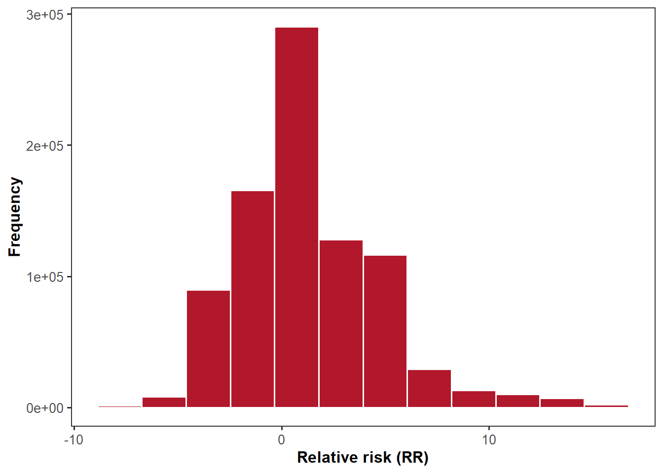

library(ggplot2)
library(dplyr)
library(scales)
library(metR)


# 2a) (optional but very useful) "trim" outliers for the color scale
#     and enforce symmetric limits around zero:
lims <- quantile(df_heat$PERC, c(0.02, 0.98), na.rm = TRUE)
max_abs <- max(abs(lims))
df_plot <- df_heat %>%
  mutate(PERC_c = pmax(pmin(PERC,  max_abs), -max_abs))

# 2b) Heatmap + countour lines
tmean_movel = df_plot %>% 
ggplot(aes(x = lag, y = tmean_val, fill = PERC_c)) +
  # interpolated raster looks smoother on screen
  geom_raster(interpolate = TRUE) +
  # contour lines (0% and ±5, ±10, ±15...)
  geom_contour(aes(z = PERC), color = "black", size = 0.25,
               breaks = c(-15, -10, -5, 0, 5, 10, 15)) +
  # label only the zero contour (neutral) to guide interpretation
  geom_text_contour(aes(z = PERC), breaks = 0, stroke = 0.15,
                    label.padding = unit(0.15, "lines"), size = 3.2) +
  # perceptual palette centered at 0 (diverging)
scale_fill_gradient2(
  low = "#2c7bb6", mid = "white", high = "#d7191c",
  midpoint = 0, limits = c(-max_abs, max_abs),
  oob = squish,
  name = "RR (%)",
  guide = guide_colorbar(
    barwidth  = unit(4, "cm"),  
    barheight = unit(0.5, "cm")
  )
)+
  #scale_x_reverse()+
  scale_x_continuous(trans = "reverse",
    breaks = pretty(df_plot$lag, n = 8), expand = c(0, 0)) +
  scale_y_continuous(breaks = pretty(df_plot$tmean_val, n = 6), expand = c(0, 0)) +
  coord_cartesian(clip = "off") +
  labs(
    x = "Lag (days)",
    y = "Temperature (°C)") +
  theme_bw(base_size = 12) +
  theme(
    panel.grid = element_blank(),
    axis.title = element_text(face = "bold", size = 12),
    axis.text  = element_text(size = 10),
    legend.title = element_text(face = "bold"),
    plot.title = element_text(face = "bold", size = 13),
    plot.subtitle = element_text(size = 10),
    legend.position = "top"
  )

tmean_movel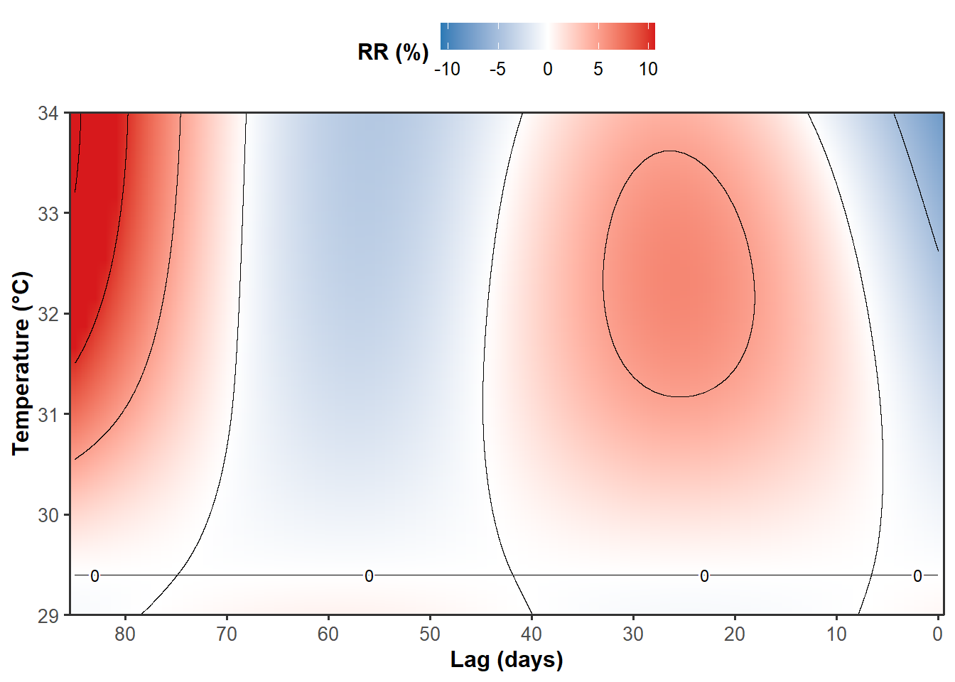

Severity

cb_cols <- names(dat)[grepl("^cb_(tmax|vpd|rain_cum)_", names(dat))]
fml_sel <- as.formula(paste("sev ~ 1 + (1|siteyear) +", paste(cb_cols, collapse = " + ")))

#dat$sev  = dat$sev/100

fit_sel <- glmmTMB::glmmTMB(
  fml_sel, data = dat,
  family = glmmTMB::beta_family(link = "logit")
)

summary(fit_sel)

 Family: beta  ( logit )
Formula:          
sev ~ 1 + (1 | siteyear) + cb_tmax_1 + cb_tmax_2 + cb_tmax_3 +  
    cb_tmax_4 + cb_tmax_5 + cb_tmax_6 + cb_tmax_7 + cb_tmax_8 +  
    cb_tmax_9 + cb_tmax_10 + cb_tmax_11 + cb_tmax_12 + cb_tmax_13 +  
    cb_tmax_14 + cb_tmax_15 + cb_tmax_16 + cb_rain_cum_1 + cb_rain_cum_2 +  
    cb_rain_cum_3 + cb_rain_cum_4 + cb_rain_cum_5 + cb_rain_cum_6 +  
    cb_rain_cum_7 + cb_rain_cum_8 + cb_rain_cum_9 + cb_rain_cum_10 +  
    cb_rain_cum_11 + cb_rain_cum_12 + cb_rain_cum_13 + cb_rain_cum_14 +  
    cb_rain_cum_15 + cb_rain_cum_16 + cb_vpd_1 + cb_vpd_2 + cb_vpd_3 +  
    cb_vpd_4 + cb_vpd_5 + cb_vpd_6 + cb_vpd_7 + cb_vpd_8 + cb_vpd_9 +  
    cb_vpd_10 + cb_vpd_11 + cb_vpd_12 + cb_vpd_13 + cb_vpd_14 +  
    cb_vpd_15 + cb_vpd_16
Data: dat

      AIC       BIC    logLik -2*log(L)  df.resid 
   -181.3      -0.9     141.6    -283.3       203 

Random effects:

Conditional model:
 Groups   Name        Variance Std.Dev.
 siteyear (Intercept) 0.1281   0.3579  
Number of obs: 254, groups:  siteyear, 199

Dispersion parameter for beta family (): 13.4 

Conditional model:
                Estimate Std. Error z value Pr(>|z|)   
(Intercept)    -91.43799   33.72773  -2.711  0.00671 **
cb_tmax_1        0.71561    0.55498   1.289  0.19725   
cb_tmax_2        0.43579    0.44981   0.969  0.33263   
cb_tmax_3       -0.32470    0.33756  -0.962  0.33610   
cb_tmax_4       -0.26453    0.50751  -0.521  0.60221   
cb_tmax_5        0.73994    0.37300   1.984  0.04728 * 
cb_tmax_6       -0.02880    0.28873  -0.100  0.92055   
cb_tmax_7       -0.13123    0.22112  -0.594  0.55284   
cb_tmax_8        0.04672    0.29409   0.159  0.87378   
cb_tmax_9        1.38327    1.13884   1.215  0.22451   
cb_tmax_10       0.86710    0.93005   0.932  0.35118   
cb_tmax_11      -0.55799    0.71165  -0.784  0.43299   
cb_tmax_12      -0.17607    1.08801  -0.162  0.87144   
cb_tmax_13       0.10668    0.47650   0.224  0.82284   
cb_tmax_14       0.31631    0.35730   0.885  0.37601   
cb_tmax_15      -0.51349    0.41931  -1.225  0.22072   
cb_tmax_16       0.05704    0.40368   0.141  0.88764   
cb_rain_cum_1   -2.19667    0.72998  -3.009  0.00262 **
cb_rain_cum_2   -1.42815    0.64735  -2.206  0.02737 * 
cb_rain_cum_3    5.09056    2.08157   2.446  0.01446 * 
cb_rain_cum_4   -3.42281    1.42454  -2.403  0.01627 * 
cb_rain_cum_5   -1.28407    0.47389  -2.710  0.00674 **
cb_rain_cum_6   -1.17585    0.50781  -2.316  0.02058 * 
cb_rain_cum_7    4.59117    1.68803   2.720  0.00653 **
cb_rain_cum_8    0.26333    1.76334   0.149  0.88129   
cb_rain_cum_9   -4.05763    1.48428  -2.734  0.00626 **
cb_rain_cum_10  -2.20038    1.90819  -1.153  0.24886   
cb_rain_cum_11 -17.85349   22.99215  -0.776  0.43745   
cb_rain_cum_12 -47.39872   34.94649  -1.356  0.17500   
cb_rain_cum_13  -0.68314    0.78249  -0.873  0.38264   
cb_rain_cum_14   0.03376    2.86137   0.012  0.99059   
cb_rain_cum_15 -48.31432   42.32921  -1.141  0.25371   
cb_rain_cum_16 -78.54418   64.56302  -1.217  0.22378   
cb_vpd_1        -0.15554    0.21531  -0.722  0.47006   
cb_vpd_2         0.13762    0.20542   0.670  0.50289   
cb_vpd_3         0.28504    0.14482   1.968  0.04905 * 
cb_vpd_4         0.14017    0.24275   0.577  0.56365   
cb_vpd_5        -0.23928    0.21029  -1.138  0.25519   
cb_vpd_6         0.31839    0.17996   1.769  0.07686 . 
cb_vpd_7        -0.14754    0.17915  -0.824  0.41018   
cb_vpd_8         0.01735    0.21960   0.079  0.93702   
cb_vpd_9        -0.42078    0.48967  -0.859  0.39017   
cb_vpd_10        0.09286    0.45933   0.202  0.83979   
cb_vpd_11        1.45724    0.49684   2.933  0.00336 **
cb_vpd_12       -0.46291    0.57102  -0.811  0.41755   
cb_vpd_13       -0.25608    0.57263  -0.447  0.65473   
cb_vpd_14       -0.70089    0.41145  -1.704  0.08848 . 
cb_vpd_15        2.27111    0.88535   2.565  0.01031 * 
cb_vpd_16       -1.09237    0.66406  -1.645  0.09997 . 
---
Signif. codes:  0 '***' 0.001 '**' 0.01 '*' 0.05 '.' 0.1 ' ' 1

# ============================================================
# PREREQUISITES (must exist in the environment):
#   fit_sel      : fitted beta-logit glmmTMB model
#   dat          : data.frame used for fitting (with cb_* columns)
#   wx_use       : weather data (epi_id, tmax, rain_cum, vpd)
#   cb_templates : list with crossbasis templates (tmax, rain_cum, vpd)
#   LAG_MAX      : maximum lag (e.g., 85)
# ============================================================

stopifnot(exists("fit_sel"), exists("dat"), exists("wx_use"),
          exists("cb_templates"), exists("LAG_MAX"))

# ------------------------------------------------------------
# 1) UTILITIES
# ------------------------------------------------------------
get_cb_names <- function(dat, var) {
  grep(paste0("^cb_", var, "_"), names(dat), value = TRUE)
}

# typical time series length per epidemic
n_ref <- wx_use %>%
  filter(!is.na(tmax)) %>%
  count(epi_id) %>%
  pull(n) %>%
  median() %>%
  as.integer()

# ensure support for all lags
n_ref <- max(n_ref, LAG_MAX + 1)

# create a daily series with value "value" only within the lag band
make_series_band <- function(value, cen, n_ref, band = NULL) {
  x <- rep(cen, n_ref)
  if (!is.null(band)) {
    lags <- 0:(n_ref - 1)
    idx  <- which(lags %in% band)
    pos  <- n_ref - idx
    x[pos] <- value
  } else {
    x[] <- value
  }
  x
}

# extract the last row of the crossbasis
last_cb_row <- function(x, cb_template, LAG_MAX) {
  cbx <- dlnm::crossbasis(
    x, lag = LAG_MAX,
    argvar = attr(cb_template, "argvar"),
    arglag = attr(cb_template, "arglag")
  )
  as.numeric(cbx[length(x), ])
}

# manual prediction (population-level; beta-logit)
predict_eta_mu <- function(bt, br, bv, beta, nm_t, nm_r, nm_v) {
  eta <- unname(beta["(Intercept)"]) +
    sum(unname(beta[nm_t]) * bt) +
    sum(unname(beta[nm_r]) * br) +
    sum(unname(beta[nm_v]) * bv)
  mu <- plogis(eta)
  c(eta = eta, mu = mu)
}

# ------------------------------------------------------------
# 2) COLUMN NAMES cb_* IN THE MODEL
# ------------------------------------------------------------
nm_t <- get_cb_names(dat, "tmax")
nm_r <- get_cb_names(dat, "rain_cum")
nm_v <- get_cb_names(dat, "vpd")
stopifnot(length(nm_t) > 0, length(nm_r) > 0, length(nm_v) > 0)

# ------------------------------------------------------------
# 3) FIXED EFFECT COEFFICIENTS
# ------------------------------------------------------------
beta <- fixef(fit_sel)$cond
stopifnot(all(c("(Intercept)", nm_t, nm_r, nm_v) %in% names(beta)))

# ------------------------------------------------------------
# 4) BASELINE (P50) FOR VARIABLES
# ------------------------------------------------------------
cen_t <- as.numeric(quantile(wx_use$tmax,     0.50, na.rm = TRUE))
cen_r <- as.numeric(quantile(wx_use$rain_cum, 0.50, na.rm = TRUE))
cen_v <- as.numeric(quantile(wx_use$vpd,      0.50, na.rm = TRUE))

# baseline series (constant)
xt0 <- make_series_band(cen_t, cen_t, n_ref, band = NULL)
xr0 <- make_series_band(cen_r, cen_r, n_ref, band = NULL)
xv0 <- make_series_band(cen_v, cen_v, n_ref, band = NULL)

bt0 <- last_cb_row(xt0, cb_templates[["tmax"]],     LAG_MAX)
br0 <- last_cb_row(xr0, cb_templates[["rain_cum"]], LAG_MAX)
bv0 <- last_cb_row(xv0, cb_templates[["vpd"]],      LAG_MAX)

# baseline severity
base <- predict_eta_mu(bt0, br0, bv0, beta, nm_t, nm_r, nm_v)
sev_base_pct <- 100 * base["mu"]

# ------------------------------------------------------------
# 5) TMAX GRID
# ------------------------------------------------------------
t_grid <- seq(19, 34, length.out = 200)

# periods
band_later   <- 0:40      # Later
band_earlier <- 41:85     # Earlier

# ------------------------------------------------------------
# 6) FUNCTION TO COMPUTE CURVES BY PERIOD
# ------------------------------------------------------------
calc_curve_phase_tmax <- function(values, band) {
  sapply(values, function(val) {

    xt <- make_series_band(value = val, cen = cen_t,
                           n_ref = n_ref, band = band)
    bt <- last_cb_row(xt, cb_templates[["tmax"]], LAG_MAX)

    pr <- predict_eta_mu(bt, br0, bv0, beta, nm_t, nm_r, nm_v)
    100 * pr["mu"]
  })
}

# ------------------------------------------------------------
# 7) COMPUTE BOTH CURVES
# ------------------------------------------------------------
sev_tmax_later   <- calc_curve_phase_tmax(t_grid, band_later)
sev_tmax_earlier <- calc_curve_phase_tmax(t_grid, band_earlier)

df_tmax <- data.frame(
  tmax = rep(t_grid, 2),
  sev_pct = c(sev_tmax_earlier, sev_tmax_later),
  phase = rep(c("Earlier", "Later"), each = length(t_grid))
)


sev_tmax = ggplot(df_tmax, aes(tmax, sev_pct, linetype = phase)) +
  #geom_hline(yintercept = 100*sev_base, linetype = 2, alpha = 0.6) +
  #geom_smooth(size = 2, se = F, color = "#B2182B") +
   geom_smooth(method = "gam",
              formula = y ~ s(x, bs = "cs", k = 2),
              se = FALSE,
              linewidth = 2, colour = "#B2182B")+
  #scale_color_brewer(palette = "Dark2") +
  labs(
    x = "Temperature (°C)",
    y = "Severity (%)",
    linetype = "Phases") +
  theme_bw(base_size = 12) +
  theme(
    legend.title = element_text(face = "bold"),
    axis.title = element_text(face = "bold", size = 12),
    axis.text  = element_text(size = 10))+
  scale_x_continuous(
    limits = c(19, 34),
    breaks = seq(19, 34, by = 3),
    expand = c(0, 0))+
   scale_y_continuous(
    limits = c(0, 100),
    breaks = seq(0, 100, by = 25),
    expand = c(0, 0))


sev_tmax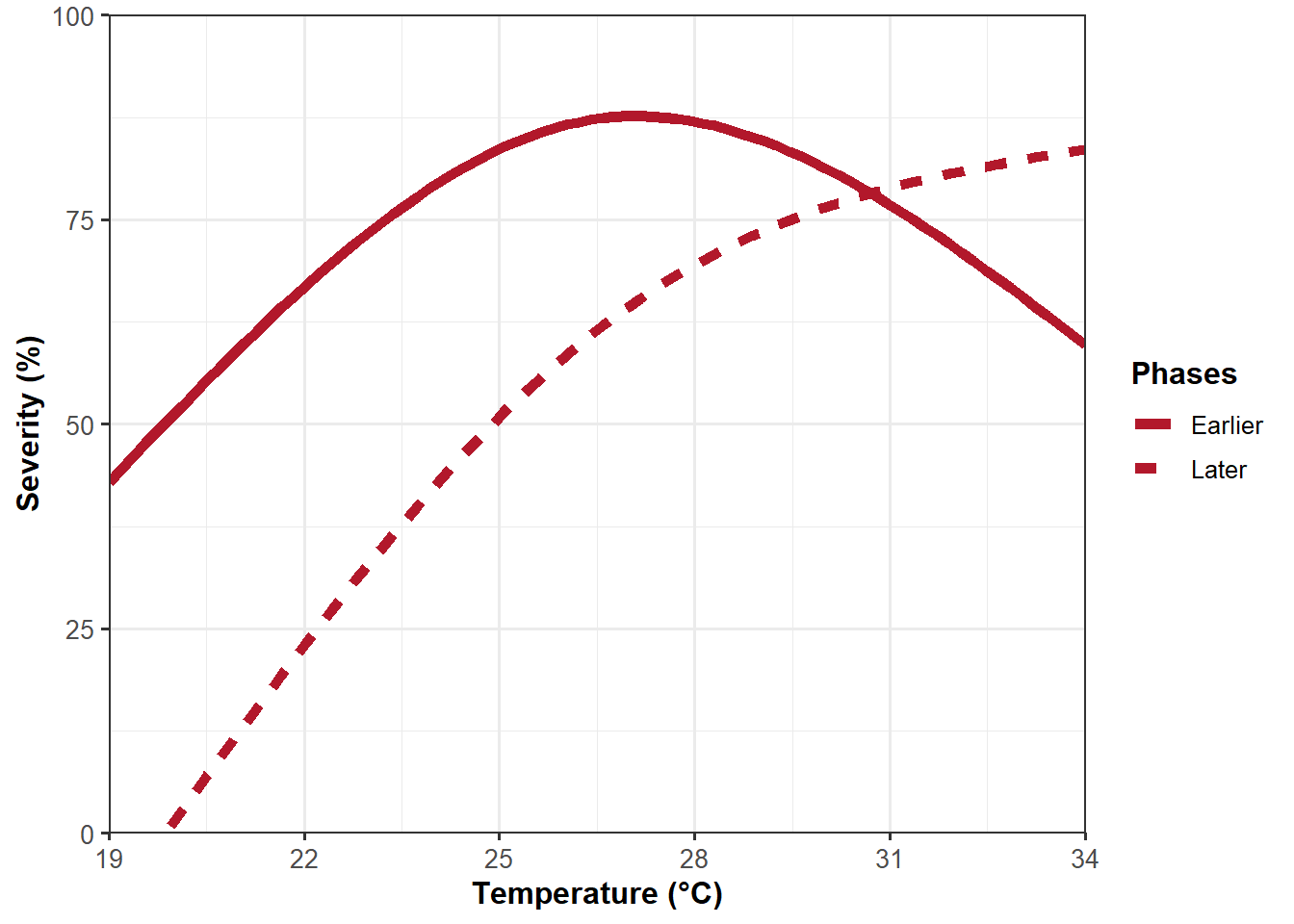

Delta

# ==============================================================
# DLNM heatmap / curves by lag bands (GLMMTMB beta-logit)
# - Effect of a single variable (e.g., tmax) across lags
# - BASELINE consistent with the DLNM "cen":
#     baseline = population-level prediction under the reference scenario:
#       tmax = P50(tmax), rain_cum = P50(rain_cum), vpd = P50(vpd)
# - Converts cumulative effect (Δη 0→L) into severity (%) via logit
# ==============================================================
# Expected inputs in the environment:
#   fit_sel      : glmmTMB beta_family(link="logit")
#   dat          : data.frame used for model fitting (contains cb_* columns)
#   cb_templates : list with crossbasis objects used in fitting (tmax, rain_cum, vpd)
#   wx_use       : data.frame/object with original time series containing epi_id and columns tmax, rain_cum, vpd
#   LAG_MAX      : maximum lag used in the crossbasis
# ==============================================================


suppressPackageStartupMessages({
  library(dlnm)
  library(glmmTMB)
  library(dplyr)
  library(tidyr)
  library(ggplot2)
  library(scales)
})

# --------------------- 0) Checks ---------------------------
stopifnot(exists("fit_sel"), exists("dat"), exists("cb_templates"), exists("wx_use"), exists("LAG_MAX"))

# --------------------- 1) Parameters --------------------------
var <- "tmax"  # tmax | rain_cum | vpd

if (is.null(cb_templates[[var]])) stop("cb_templates[['", var, "']] does not exist.")
if (!all(c("tmax","rain_cum","vpd") %in% names(cb_templates))) {
  stop("cb_templates must contain: 'tmax', 'rain_cum', 'vpd'.")
}

x_all <- wx_use[[var]]
if (is.null(x_all)) stop("wx_use[['", var, "']] não existe.")

# DLNM "cen": P50 of the target variable
P50_var <- as.numeric(quantile(x_all, 0.50, na.rm = TRUE))

at_vals <- seq(19, 34, length.out = 1000) 

# (optional) Warning if extrapolation occurs beyond observed range
rng_obs <- range(x_all, na.rm = TRUE)
if (min(at_vals) < rng_obs[1] || max(at_vals) > rng_obs[2]) {
  message("WARNING: at_vals includes values outside the observed range: ",
          "observed range = [", round(rng_obs[1],2), ", ", round(rng_obs[2],2), "]")
}

# Lags for plotting
lag_max_plot <- 85L
lag_max_plot <- min(lag_max_plot, LAG_MAX)

# --------------------- 2) Coefs/VCOV only for cb_var block ------------------
cb <- cb_templates[[var]]

cf_all <- coef(summary(fit_sel))$cond[, 1]
vc_all <- vcov(fit_sel)$cond

pref <- paste0("^cb_", var, "_")

idx_beta <- grep(pref, names(cf_all))
if (length(idx_beta) == 0) stop("Could not find cb_ coefficients for var='", var, "'.")
beta <- cf_all[idx_beta]

idx_rows <- grep(pref, rownames(vc_all))
idx_cols <- grep(pref, colnames(vc_all))
V <- vc_all[idx_rows, idx_cols, drop = FALSE]

# Checks
if (length(beta) != ncol(cb)) stop("length(beta) != ncol(cb).  Check cb_templates and the model.")
if (!(nrow(V) == ncol(cb) && ncol(V) == ncol(cb))) stop("VCOV does not match ncol(cb).")

# --------------------- 3) crosspred: Δη by lag vs cen=P50_var ----------------
cp <- dlnm::crosspred(
  cb,
  coef  = beta,
  vcov  = V,
  at    = at_vals,
  cen   = P50_var,
  bylag = 1
)

mf <- cp$matfit  # Δη (link) by lag; rows=at_vals, columns=lags

# Sort lags
lag_idx <- suppressWarnings(as.integer(gsub("lag", "", colnames(mf))))
if (anyNA(lag_idx)) {
  lag_idx <- 0:(ncol(mf) - 1)
  colnames(mf) <- paste0("lag", lag_idx)
}
ord <- order(lag_idx)
mf <- mf[, ord, drop = FALSE]
lag_idx <- lag_idx[ord]

# keep 0..lag_max_plot
keep <- which(lag_idx >= 0 & lag_idx <= lag_max_plot)
mf <- mf[, keep, drop = FALSE]
lag_idx <- lag_idx[keep]

# --------------------- 4) Consistent baseline (joint P50 scenario) ------------
P50_t <- as.numeric(quantile(wx_use[["tmax"]],     0.50, na.rm = TRUE))
P50_r <- as.numeric(quantile(wx_use[["rain_cum"]], 0.50, na.rm = TRUE))
P50_v <- as.numeric(quantile(wx_use[["vpd"]],      0.50, na.rm = TRUE))

# n_ref (typical series length)
n_ref <- wx_use %>%
  filter(!is.na(tmax)) %>%
  count(epi_id) %>%
  pull(n) %>%
  stats::median() %>%
  as.integer()

n_ref <- max(n_ref, LAG_MAX + 1)

# cb_* names in dat
nm_t <- grep("^cb_tmax_",     names(dat), value = TRUE)
nm_r <- grep("^cb_rain_cum_", names(dat), value = TRUE)
nm_v <- grep("^cb_vpd_",      names(dat), value = TRUE)
stopifnot(length(nm_t) > 0, length(nm_r) > 0, length(nm_v) > 0)

# function: last crossbasis row for constant series
last_cb_row_const <- function(value, cb_template, LAG_MAX, n_ref) {
  x <- rep(value, n_ref)
  cbx <- dlnm::crossbasis(
    x, lag = LAG_MAX,
    argvar = attr(cb_template, "argvar"),
    arglag = attr(cb_template, "arglag")
  )
  as.numeric(cbx[n_ref, ])
}

bt0 <- last_cb_row_const(P50_t, cb_templates[["tmax"]],     LAG_MAX, n_ref)
br0 <- last_cb_row_const(P50_r, cb_templates[["rain_cum"]], LAG_MAX, n_ref)
bv0 <- last_cb_row_const(P50_v, cb_templates[["vpd"]],      LAG_MAX, n_ref)

# reference newdata
nd0 <- data.frame(siteyear = dat$siteyear[1])  # must contain a valid level
nd0[nm_t] <- as.list(bt0)
nd0[nm_r] <- as.list(br0)
nd0[nm_v] <- as.list(bv0)

sev_base <- as.numeric(predict(fit_sel, newdata = nd0, type = "response", re.form = NA))

# --------------------- 5) Convert cumulative Δη 0→L into final severity -----
mf_cum <- t(apply(mf, 1, cumsum))

SEV_mat <- plogis(qlogis(sev_base) + mf_cum)   # 0–1
SEVdiff_pp <- 100 * (SEV_mat - sev_base)       # percent points (pp)

# --------------------- 6) Long data frame (heatmap) ---------------------------
df_diff <- as.data.frame(100 * (SEV_mat - sev_base))
colnames(df_diff) <- paste0("lag_", lag_idx)

df_diff <- df_diff %>%
  mutate(var_val = at_vals) %>%
  pivot_longer(starts_with("lag_"), names_to = "lag", values_to = "SEV_diff_pp") %>%
  mutate(lag = as.integer(gsub("lag_", "", lag)))

# --------------------- 7) Heatmap (Δ in pp) ----------------------------------
p_heat_diff_tmax <- ggplot(df_diff, aes(x = lag, y = var_val, fill = SEV_diff_pp)) +
  geom_raster() +
  scale_fill_viridis_c(name = "Δ (pp)") +
  labs(
    x = "Lag (days)",
    y = " Temperature (°C)") +
  theme_bw(base_size = 12) +
  theme(plot.title = element_text(face = "bold"),
        axis.title = element_text(face = "bold"))+
  scale_x_continuous(
    trans = "reverse",
    breaks = c(0,10,20,30,40,50,60,70,80),
    limits = c(0,85),
    expand = c(0, 0)
  ) +
  scale_y_continuous(
    limits = c(19, 34),
    breaks = seq(19, 35, by = 3),
    expand = c(0, 0))

print(p_heat_diff_tmax)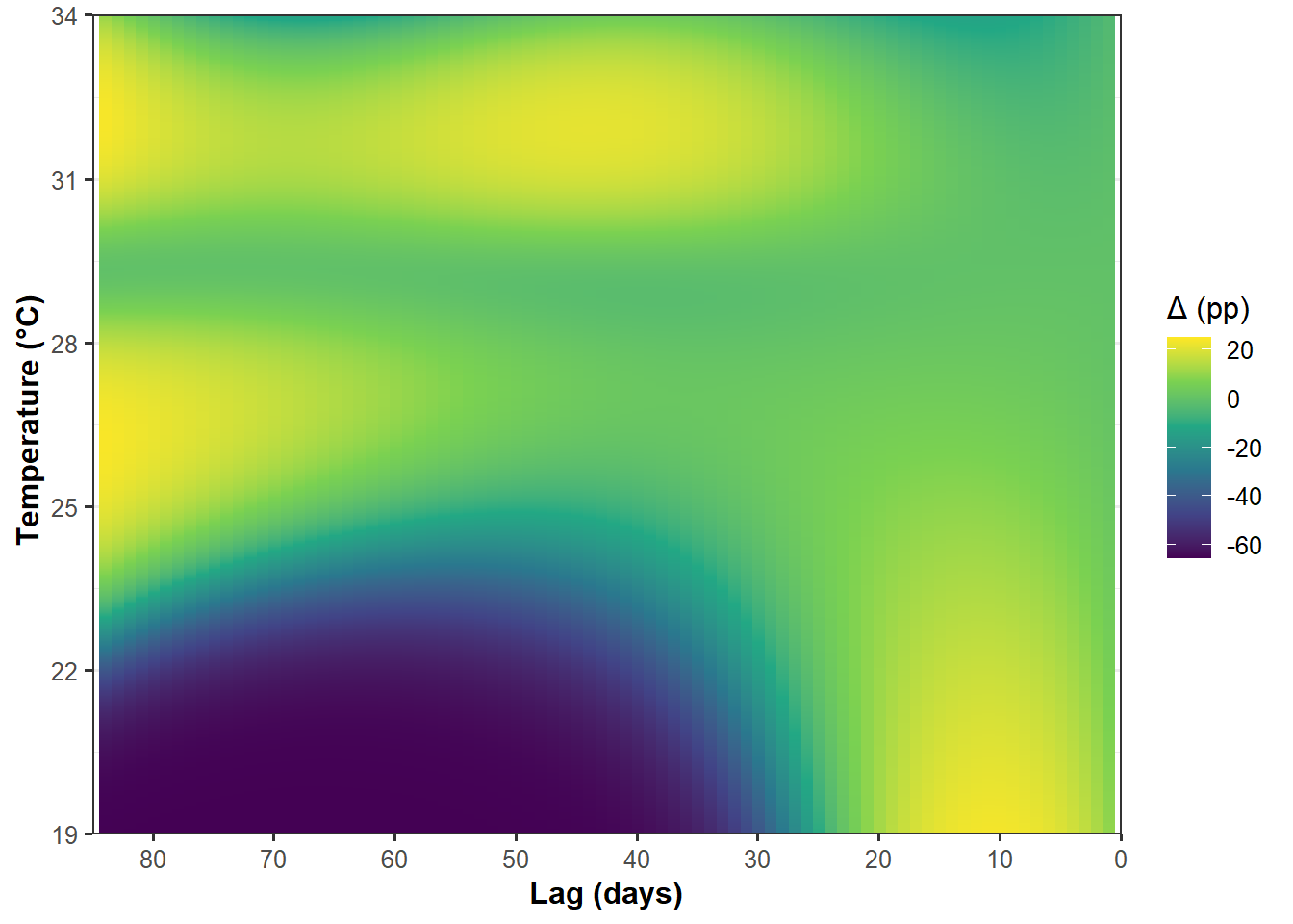

Precipitation

library(dlnm)
library(dplyr)
library(ggplot2)
library(tidyr)

# ==============================================================
# 1) EXTRACT COEFFICIENTS
# ==============================================================

var <- "rain_cum"
cb  <- cb_templates[[var]]

cf  <- coef(summary(fit_tmb))$cond[,1]
vc  <- vcov(fit_tmb)$cond

idx     <- grepl("^cb_rain_cum_", names(cf))
beta    <- cf[idx]
vc_sub  <- vc[idx, idx]

stopifnot(length(beta) == ncol(cb))
stopifnot(nrow(vc_sub) == ncol(cb))

# ==============================================================
# 2) DEFINE GRID AND TMEAN RANGE FOR THE HEATMAP
# ==============================================================

x_all <- wx_use[[var]]
P50   <- quantile(x_all, 0.50, na.rm = TRUE)

# Grid used by DLNM
grid <- sort(unique(as.numeric(quantile(
  x_all, seq(0.05, 0.95, by = 0.01), na.rm = TRUE
))))

# Desired values for the heatmap (0 to 600 mm)
#at_vals <- seq(1, 2, length.out = 10000)
at_vals <- seq(0, 600, length.out = 10000)

# Adjust to the REAL grid range (avoids extrapolation)
at_vals <- at_vals[at_vals >= min(grid) & at_vals <= max(grid)]

# ==============================================================
# 3) crosspred IN ALL at-vals (mobile lag)
# ==============================================================

cp <- crosspred(
  cb,
  coef  = beta,
  vcov  = vc_sub,
  at    = at_vals,
  cen   = P50,
  bylag = 1
)

# matrix: rows = tmean values; columns = lags
mf <- cp$matfit

# create lag vectors
lag_idx <- suppressWarnings(as.integer(gsub("lag","",colnames(mf))))
if (anyNA(lag_idx)) lag_idx <- 0:(ncol(mf)-1)

# ==============================================================
# 4) Convert to RR (lag) and then % (% change)
# ==============================================================

RR_mat   <- exp(mf)
PERC_mat <- (RR_mat - 1) * 100

# pivot for tidy format
df_heat <- as.data.frame(PERC_mat)
colnames(df_heat) <- paste0("lag_", lag_idx)
df_heat <- df_heat %>%
  mutate(tmean_val = at_vals) %>%
  pivot_longer(cols = starts_with("lag_"),
               names_to = "lag",
               values_to = "PERC") %>%
  mutate(lag = as.integer(gsub("lag_", "", lag)))

freq_rain = df_heat %>% 
  ggplot(aes(PERC))+
  geom_histogram(bins = 12, color = "white", fill = "#2166AC")+
  theme_bw(base_size = 12) +
    theme(
    panel.grid = element_blank(),
    axis.title = element_text(face = "bold", size = 12),
    axis.text  = element_text(size = 10),
    legend.title = element_text(face = "bold"),
    plot.title = element_text(face = "bold", size = 13),
    plot.subtitle = element_text(size = 10),
    legend.position = "top"
  )+
  labs(
    x = "Relative risk (RR)",
    y = "Frequency"
  )

freq_rain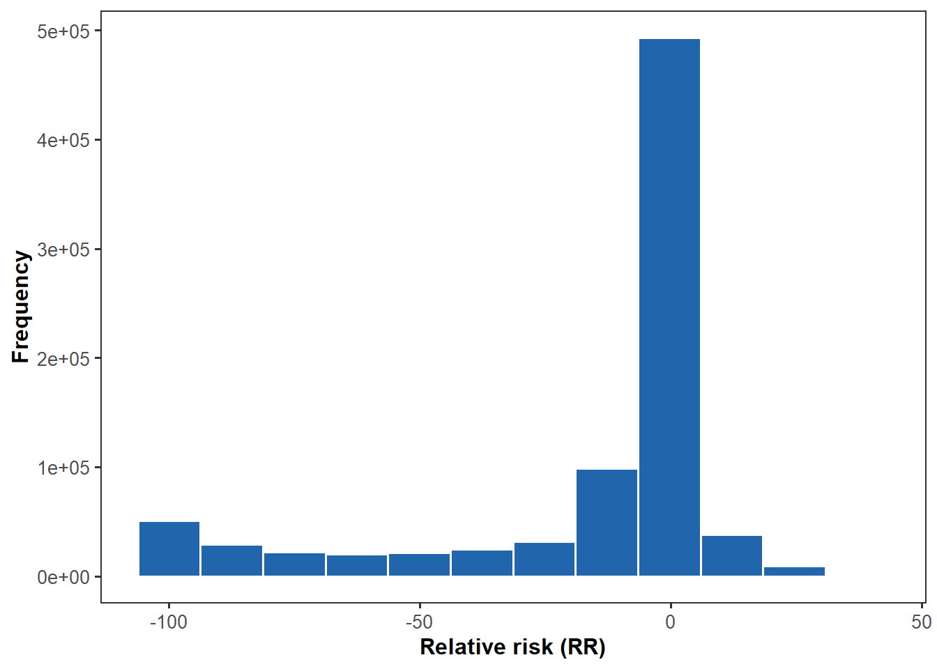

library(ggplot2)
library(dplyr)
library(scales)

# 2a) (optional but very useful) "trim" outliers for the color scale
#     and enforce symmetric limits around zero:
lims <- quantile(df_heat$PERC, c(0.02, 0.98), na.rm = TRUE)
max_abs <- max(abs(lims))
df_plot <- df_heat %>%
  mutate(PERC_c = pmax(pmin(PERC,  max_abs), -max_abs))

# 2b) Heatmap + countour lines
rain_movel = df_plot %>% 
ggplot(aes(x = lag, y = tmean_val, fill = PERC_c)) +
  # interpolated raster looks smoother on screen
  geom_raster(interpolate = TRUE) +
  # contour lines (0% and ±5, ±10, ±15...)
  geom_contour(aes(z = PERC), color = "black", size = 0.25) +
  # label only the zero contour (neutral) to guide interpretation
  geom_text_contour(aes(z = PERC), breaks = 0, stroke = 0.15,
                    label.padding = unit(0.15, "lines"), size = 3.2) +
  # perceptual palette centered at 0 (diverging)
scale_fill_gradient2(
  low = "#2c7bb6", mid = "white", high = "#d7191c",
  midpoint = 0, limits = c(-max_abs, max_abs),
  oob = squish,
  name = "RR (%)",
  guide = guide_colorbar(
    barwidth  = unit(4, "cm"),  
    barheight = unit(0.5, "cm")  
  )
)+
  scale_x_continuous(trans = "reverse",
    breaks = pretty(df_plot$lag, n = 8), expand = c(0, 0)) +
  scale_y_continuous(breaks = pretty(df_plot$tmean_val, n = 6), expand = c(0, 0)) +
  coord_cartesian(clip = "off") +
  labs(
    x = "Lag (days)",
    y = "Precipitation (mm)") +
  theme_bw(base_size = 12) +
  theme(
    panel.grid = element_blank(),
    axis.title = element_text(face = "bold", size = 12),
    axis.text  = element_text(size = 10),
    legend.title = element_text(face = "bold"),
    plot.title = element_text(face = "bold", size = 13),
    plot.subtitle = element_text(size = 10),
    legend.position = "top")+
  scale_y_continuous(
    limits = c(0, 600),
    breaks = seq(0, 600, by = 100),
    expand = c(0, 0))

rain_movel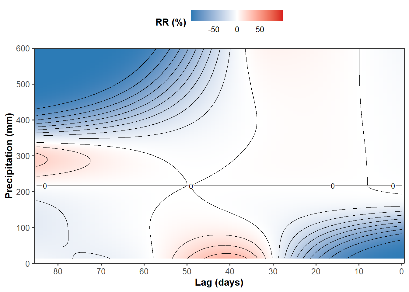

Severity

suppressPackageStartupMessages({
  library(dplyr)
  library(dlnm)
  library(glmmTMB)
  library(ggplot2)
})

# ============================================================
# PREREQUISITES (must exist in the environment):
#   fit_sel      : fitted beta-logit glmmTMB model
#   dat          : data.frame used for fitting (with cb_* columns)
#   wx_use       : weather data (epi_id, tmax, rain_cum, vpd)
#   cb_templates : list with crossbasis templates (tmax, rain_cum, vpd)
#   LAG_MAX      : maximum lag (e.g., 85)
# ============================================================
stopifnot(exists("fit_sel"), exists("dat"), exists("wx_use"),
          exists("cb_templates"), exists("LAG_MAX"))

# ------------------------------------------------------------
# 1) UTILITIES
# ------------------------------------------------------------
get_cb_names <- function(dat, var) {
  grep(paste0("^cb_", var, "_"), names(dat), value = TRUE)
}

# typical time series length per epidemic
n_ref <- wx_use %>%
  filter(!is.na(rain_cum)) %>%
  count(epi_id) %>%
  pull(n) %>%
  median() %>%
  as.integer()

# ensure support for all lags
n_ref <- max(n_ref, LAG_MAX + 1)

# create a daily series with value "value" only within the lag band
make_series_band <- function(value, cen, n_ref, band = NULL) {
  x <- rep(cen, n_ref)
  if (!is.null(band)) {
    lags <- 0:(n_ref - 1)
    idx  <- which(lags %in% band)
    pos  <- n_ref - idx
    x[pos] <- value
  } else {
    x[] <- value
  }
  x
}

# extract the last row of the crossbasis
last_cb_row <- function(x, cb_template, LAG_MAX) {
  cbx <- dlnm::crossbasis(
    x, lag = LAG_MAX,
    argvar = attr(cb_template, "argvar"),
    arglag = attr(cb_template, "arglag")
  )
  as.numeric(cbx[length(x), ])
}

# manual prediction (population-level; beta-logit)
predict_eta_mu <- function(bt, br, bv, beta, nm_t, nm_r, nm_v) {
  eta <- unname(beta["(Intercept)"]) +
    sum(unname(beta[nm_t]) * bt) +
    sum(unname(beta[nm_r]) * br) +
    sum(unname(beta[nm_v]) * bv)
  mu <- plogis(eta)
  c(eta = eta, mu = mu)
}

# ------------------------------------------------------------
# 2) COLUMN NAMES cb_* IN THE MODEL
# ------------------------------------------------------------
nm_t <- get_cb_names(dat, "tmax")
nm_r <- get_cb_names(dat, "rain_cum")
nm_v <- get_cb_names(dat, "vpd")
stopifnot(length(nm_t) > 0, length(nm_r) > 0, length(nm_v) > 0)

# ------------------------------------------------------------
# 3) FIXED EFFECT COEFFICIENTS
# ------------------------------------------------------------
beta <- fixef(fit_sel)$cond
stopifnot(all(c("(Intercept)", nm_t, nm_r, nm_v) %in% names(beta)))

# ------------------------------------------------------------
# 4) BASELINE (P50) FOR VARIABLES
# ------------------------------------------------------------
cen_t <- as.numeric(quantile(wx_use$tmax,     0.50, na.rm = TRUE))
cen_r <- as.numeric(quantile(wx_use$rain_cum, 0.50, na.rm = TRUE))
cen_v <- as.numeric(quantile(wx_use$vpd,      0.50, na.rm = TRUE))

# baseline series
xt0 <- make_series_band(cen_t, cen_t, n_ref, band = NULL)
xr0 <- make_series_band(cen_r, cen_r, n_ref, band = NULL)
xv0 <- make_series_band(cen_v, cen_v, n_ref, band = NULL)

bt0 <- last_cb_row(xt0, cb_templates[["tmax"]],     LAG_MAX)
br0 <- last_cb_row(xr0, cb_templates[["rain_cum"]], LAG_MAX)
bv0 <- last_cb_row(xv0, cb_templates[["vpd"]],      LAG_MAX)

# baseline severity
base <- predict_eta_mu(bt0, br0, bv0, beta, nm_t, nm_r, nm_v)
sev_base_pct <- 100 * base["mu"]

# ------------------------------------------------------------
# 5) RAIN CUM GRID
# ------------------------------------------------------------
r_grid <- seq(0, 600, length.out = 200)

# periods
band_later   <- 0:40      # Later
band_earlier <- 41:85     # Earlier

# ------------------------------------------------------------
# 6) FUNCTION TO COMPUTE CURVES BY PERIOD
# ------------------------------------------------------------
calc_curve_phase_rain <- function(values, band) {
  sapply(values, function(val) {

    xr <- make_series_band(
      value = val,
      cen   = cen_r,
      n_ref = n_ref,
      band  = band
    )

    br <- last_cb_row(xr, cb_templates[["rain_cum"]], LAG_MAX)

    pr <- predict_eta_mu(bt0, br, bv0, beta, nm_t, nm_r, nm_v)

    100 * pr["mu"]
  })
}

# ------------------------------------------------------------
# 7) COMPUTE BOTH CURVES
# ------------------------------------------------------------
sev_rain_later   <- calc_curve_phase_rain(r_grid, band_later)
sev_rain_earlier <- calc_curve_phase_rain(r_grid, band_earlier)

df_rain <- data.frame(
  rain_cum = rep(r_grid, 2),
  sev_pct = c(sev_rain_earlier, sev_rain_later),
  phase = rep(c("Earlier", "Later"), each = length(r_grid))
)


sev_rain = ggplot(df_rain, aes(rain_cum, sev_pct, linetype = phase)) +
  #geom_hline(yintercept = 100*sev_base, linetype = 2, alpha = 0.6) +
  #geom_smooth(size = 2, se = F, colour = "#2166AC") +
  geom_smooth(method = "gam",
              formula = y ~ s(x, bs = "cs", k = 2),
              se = FALSE,
              linewidth = 2, colour = "#2166AC")+
  #scale_color_brewer(palette = "Dark2") +
  labs(
    x = "Precipitation (mm)",
    y = "Severity (%)",
    linetype = "Phases") +
  theme_bw(base_size = 12) +
  theme(
    legend.title = element_text(face = "bold"),
    axis.title = element_text(face = "bold", size = 12),
    axis.text  = element_text(size = 10))+
  scale_x_continuous(
    limits = c(0, 600),
    breaks = seq(0, 600, by = 100),
    expand = c(0, 0))+
   scale_y_continuous(
    limits = c(0, 100),
    breaks = seq(0, 100, by = 25),
    expand = c(0, 0))

sev_rain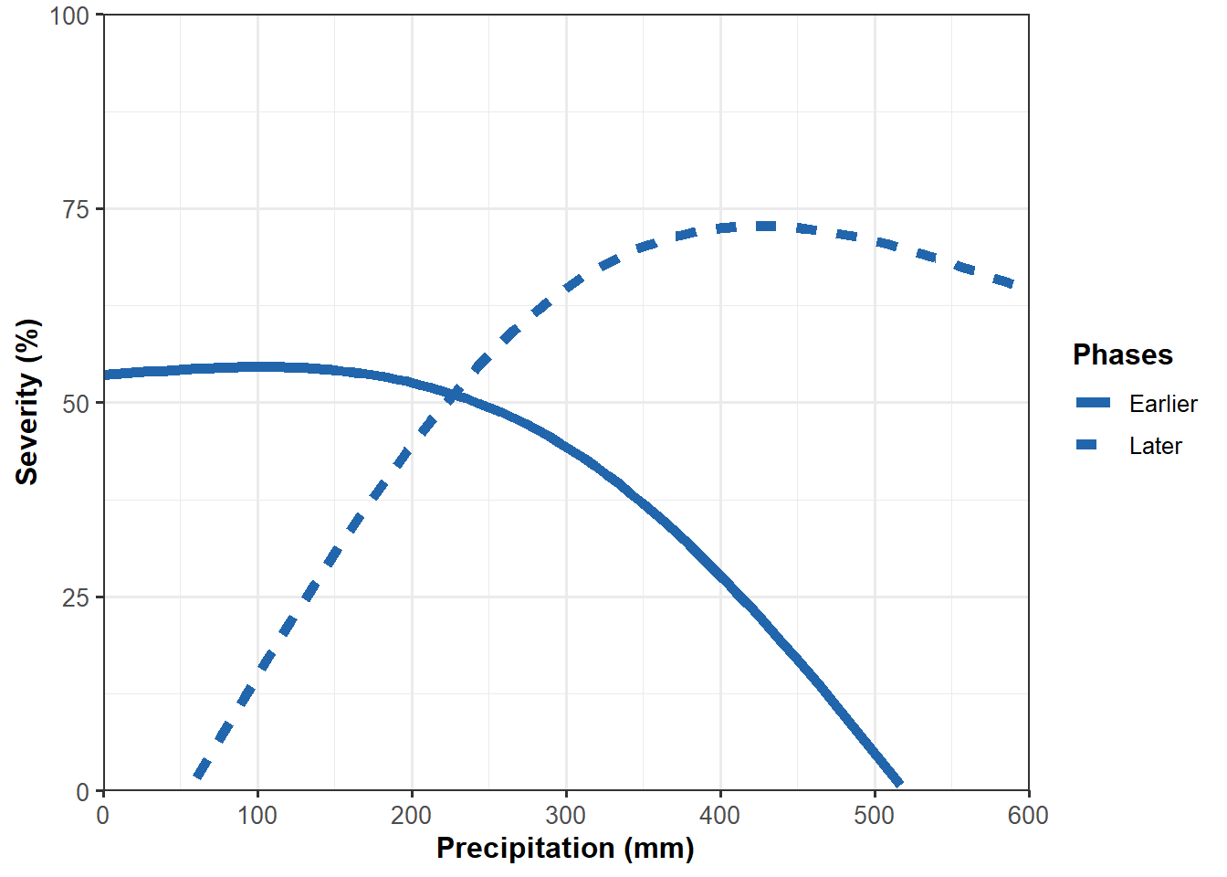

Delta

# ==============================================================
# DLNM heatmap / curves by lag bands (GLMMTMB beta-logit)
# - Effect of a single variable (e.g., tmax) across lags
# - BASELINE consistent with the DLNM "cen":
#     baseline = population-level prediction under the reference scenario:
#       tmax = P50(tmax), rain_cum = P50(rain_cum), vpd = P50(vpd)
# - Converts cumulative effect (Δη 0→L) into severity (%) via logit
# ==============================================================
# Expected inputs in the environment:
#   fit_sel      : glmmTMB beta_family(link="logit")
#   dat          : data.frame used for model fitting (contains cb_* columns)
#   cb_templates : list with crossbasis objects used in fitting (tmax, rain_cum, vpd)
#   wx_use       : data.frame/object with original time series containing epi_id and columns tmax, rain_cum, vpd
#   LAG_MAX      : maximum lag used in the crossbasis
# ==============================================================

suppressPackageStartupMessages({
  library(dlnm)
  library(glmmTMB)
  library(dplyr)
  library(tidyr)
  library(ggplot2)
  library(scales)
})

# --------------------- 0) Checks ---------------------------
stopifnot(exists("fit_sel"), exists("dat"), exists("cb_templates"), exists("wx_use"), exists("LAG_MAX"))

# --------------------- 1) Parameters --------------------------
var <- "rain_cum" 

if (is.null(cb_templates[[var]])) stop("cb_templates[['", var, "']] does not exist.")
if (!all(c("tmax","rain_cum","vpd") %in% names(cb_templates))) {
  stop("cb_templates must contain: 'tmax', 'rain_cum', 'vpd'.")
}


x_all <- wx_use[[var]]
if (is.null(x_all)) stop("wx_use[['", var, "']] does not exist.")

# DLNM "cen": P50 of the target variable
P50_var <- as.numeric(quantile(x_all, 0.50, na.rm = TRUE))

# trim the range to the observed interval to avoid extrapolation
grid_obs <- sort(unique(as.numeric(quantile(x_all, seq(0.05, 0.95, by = 0.01), na.rm = TRUE))))
at_vals  <- seq(0, 600, length.out = 1000)
at_vals  <- at_vals[at_vals >= min(grid_obs) & at_vals <= max(grid_obs)]
if (length(at_vals) < 5) stop("at_vals it became too short after trimming. Adjustment seq().")

# Lags for plotting
lag_max_plot <- 85L                 
lag_max_plot <- min(lag_max_plot, LAG_MAX)

# --------------------- 2) Coefs/VCOV only for cb_var block ------------------
cb <- cb_templates[[var]]

cf_all <- coef(summary(fit_sel))$cond[, 1]
vc_all <- vcov(fit_sel)$cond

pref <- paste0("^cb_", var, "_")

idx_beta <- grep(pref, names(cf_all))
if (length(idx_beta) == 0) stop("Could not find cb_ coefficients for var='", var, "'.")
beta <- cf_all[idx_beta]

idx_rows <- grep(pref, rownames(vc_all))
idx_cols <- grep(pref, colnames(vc_all))
V <- vc_all[idx_rows, idx_cols, drop = FALSE]

# Checks
if (length(beta) != ncol(cb)) stop("length(beta) != ncol(cb). Check cb_templates and the model.")
if (!(nrow(V) == ncol(cb) && ncol(V) == ncol(cb))) stop("VCOV does not match ncol(cb).")

# --------------------- 3) crosspred: Δη by lag vs cen=P50_var ----------------
cp <- dlnm::crosspred(
  cb,
  coef  = beta,
  vcov  = V,
  at    = at_vals,
  cen   = P50_var,
  bylag = 1
)

mf <- cp$matfit  # Δη (link) by lag; rows=at_vals, columns=lags

# Sort lags
lag_idx <- suppressWarnings(as.integer(gsub("lag", "", colnames(mf))))
if (anyNA(lag_idx)) {
  lag_idx <- 0:(ncol(mf) - 1)
  colnames(mf) <- paste0("lag", lag_idx)
}
ord <- order(lag_idx)
mf <- mf[, ord, drop = FALSE]
lag_idx <- lag_idx[ord]

# keep 0..lag_max_plot
keep <- which(lag_idx >= 0 & lag_idx <= lag_max_plot)
mf <- mf[, keep, drop = FALSE]
lag_idx <- lag_idx[keep]

# --------------------- 4) Consistent baseline (joint P50 scenario) ------------
# References (P50) for ALL model variables
P50_t <- as.numeric(quantile(wx_use[["tmax"]],     0.50, na.rm = TRUE))
P50_r <- as.numeric(quantile(wx_use[["rain_cum"]], 0.50, na.rm = TRUE))
P50_v <- as.numeric(quantile(wx_use[["vpd"]],      0.50, na.rm = TRUE))

# n_ref (typical series length)
n_ref <- wx_use %>%
  filter(!is.na(tmax)) %>%
  count(epi_id) %>%
  pull(n) %>%
  stats::median() %>%
  as.integer()

# cb_* names in dat
nm_t <- grep("^cb_tmax_",     names(dat), value = TRUE)
nm_r <- grep("^cb_rain_cum_", names(dat), value = TRUE)
nm_v <- grep("^cb_vpd_",      names(dat), value = TRUE)

stopifnot(length(nm_t) > 0, length(nm_r) > 0, length(nm_v) > 0)

# function: last crossbasis row for constant series
last_cb_row <- function(value, cb_template, LAG_MAX, n_ref) {
  x <- rep(value, n_ref)
  cbx <- dlnm::crossbasis(
    x, lag = LAG_MAX,
    argvar = attr(cb_template, "argvar"),
    arglag = attr(cb_template, "arglag")
  )
  as.numeric(cbx[n_ref, ])
}

# cb "last line" in the reference scenario
bt0 <- last_cb_row(P50_t, cb_templates[["tmax"]],     LAG_MAX, n_ref)
br0 <- last_cb_row(P50_r, cb_templates[["rain_cum"]], LAG_MAX, n_ref)
bv0 <- last_cb_row(P50_v, cb_templates[["vpd"]],      LAG_MAX, n_ref)

# reference newdata
nd0 <- data.frame(siteyear = NA)
nd0[nm_t] <- as.list(bt0)
nd0[nm_r] <- as.list(br0)
nd0[nm_v] <- as.list(bv0)

# baseline pop-level (random effects set to zero)
sev_base <- as.numeric(predict(fit_sel, newdata = nd0, type = "response", re.form = NA))

# --------------------- 5) Convert cumulative Δη 0→L into final severity -----
mf_cum <- t(apply(mf, 1, cumsum))

SEV_mat <- plogis(qlogis(sev_base) + mf_cum)      # 0–1
SEVpct_mat <- 100 * SEV_mat                       # 0–100

# (Optional) Absolute difference vs. baseline (in percentage points)
SEVdiffpct_mat <- 100 * (SEV_mat - sev_base)

# (optional) Accumulated Odds Ratio (logit): OR = exp(Δη_cum)
OR_mat <- exp(mf_cum)

# --------------------- 6) Data frames long (heatmap) -------------------------
df_sev <- as.data.frame(SEVpct_mat)
colnames(df_sev) <- paste0("lag_", lag_idx)

df_sev <- df_sev %>%
  mutate(var_val = at_vals) %>%
  pivot_longer(starts_with("lag_"), names_to = "lag", values_to = "SEV_pct") %>%
  mutate(lag = as.integer(gsub("lag_", "", lag)))

df_diff <- as.data.frame(SEVdiffpct_mat)
colnames(df_diff) <- paste0("lag_", lag_idx)

df_diff <- df_diff %>%
  mutate(var_val = at_vals) %>%
  pivot_longer(starts_with("lag_"), names_to = "lag", values_to = "SEV_diff_pp") %>%
  mutate(lag = as.integer(gsub("lag_", "", lag)))


p_heat_diff_rain <- ggplot(df_diff, aes(x = lag, y = var_val, fill = SEV_diff_pp)) +
  geom_raster() +
  scale_fill_viridis_c(name = "Δ (pp)") +
  labs(
    x = "Lag (days)",
    y = " Precipitation (mm)") +
  theme_bw(base_size = 12) +
  theme(plot.title = element_text(face = "bold"),
        axis.title = element_text(face = "bold"))+
  scale_x_continuous(
    trans = "reverse",
    breaks = c(0,10,20,30,40,50,60,70,80),
    limits = c(0,85),
    expand = c(0, 0)
  ) +
  scale_y_continuous(
    limits = c(0, 600),
    breaks = seq(0, 600, by = 100),
    expand = c(0, 0))

print(p_heat_diff_rain)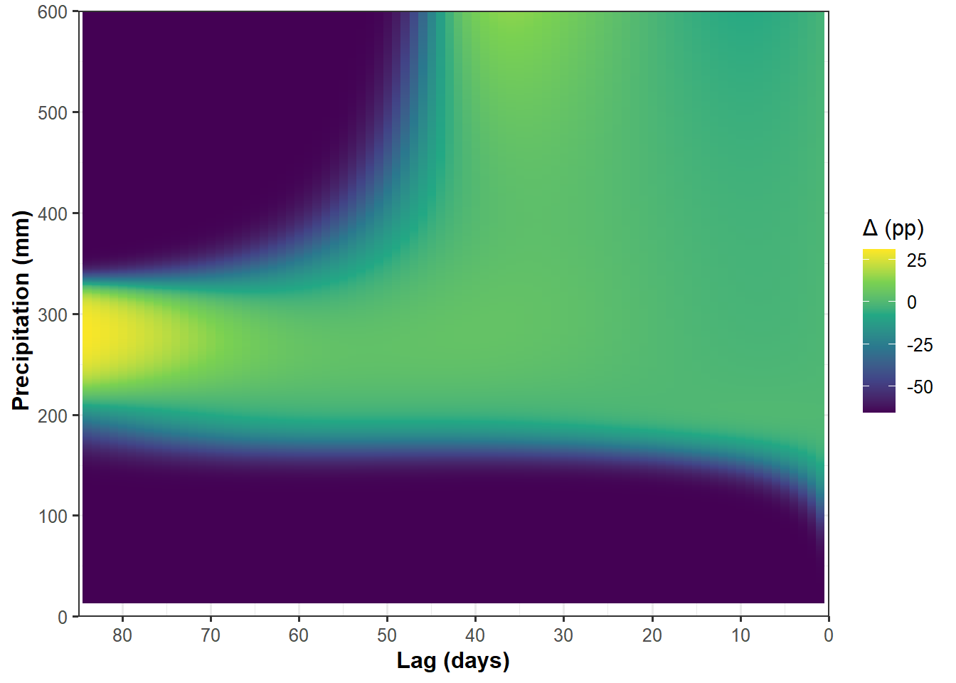

VPD

library(dlnm)
library(dplyr)
library(ggplot2)
library(tidyr)

# ==============================================================
# 1) EXTRACT COEFFICIENTS
# ==============================================================

var <- "vpd"
cb  <- cb_templates[[var]]

cf  <- coef(summary(fit_tmb))$cond[,1]
vc  <- vcov(fit_tmb)$cond

idx     <- grepl("^cb_vpd_", names(cf))
beta    <- cf[idx]
vc_sub  <- vc[idx, idx]

stopifnot(length(beta) == ncol(cb))
stopifnot(nrow(vc_sub) == ncol(cb))

# ==============================================================
# 2) DEFINE GRID AND TMEAN RANGE FOR THE HEATMAP
# ==============================================================

x_all <- wx_use[[var]]
P50   <- quantile(x_all, 0.50, na.rm = TRUE)

# Grid used by DLNM
grid <- sort(unique(as.numeric(quantile(
  x_all, seq(0.05, 0.95, by = 0.01), na.rm = TRUE
))))

# Desired values for the heatmap (0.5 to 1.5 kPa)
#at_vals <- seq(1, 2, length.out = 10000)
at_vals <- seq(0.50, 1.5, length.out = 10000)

# Adjust to the REAL grid range (avoids extrapolation)
at_vals <- at_vals[at_vals >= min(grid) & at_vals <= max(grid)]

# ==============================================================
# 3) crosspred IN ALL at-vals (mobile lag)
# ==============================================================

cp <- crosspred(
  cb,
  coef  = beta,
  vcov  = vc_sub,
  at    = at_vals,
  cen   = P50,
  bylag = 1
)

# matrix: rows = tmean values; columns = lags
mf <- cp$matfit

# create lag vectors
lag_idx <- suppressWarnings(as.integer(gsub("lag","",colnames(mf))))
if (anyNA(lag_idx)) lag_idx <- 0:(ncol(mf)-1)

# ==============================================================
# 4) Convert to RR (lag) and then % (% change)
# ==============================================================

RR_mat   <- exp(mf)
PERC_mat <- (RR_mat - 1) * 100

# pivô para formato tidy
df_heat <- as.data.frame(PERC_mat)
colnames(df_heat) <- paste0("lag_", lag_idx)
df_heat <- df_heat %>%
  mutate(tmean_val = at_vals) %>%
  pivot_longer(cols = starts_with("lag_"),
               names_to = "lag",
               values_to = "PERC") %>%
  mutate(lag = as.integer(gsub("lag_", "", lag)))

freq_vpd = df_heat %>% 
  ggplot(aes(PERC))+
  geom_histogram(bins = 12, color = "white", fill = "green4")+
  theme_bw(base_size = 12) +
    theme(
    panel.grid = element_blank(),
    axis.title = element_text(face = "bold", size = 12),
    axis.text  = element_text(size = 10),
    legend.title = element_text(face = "bold"),
    plot.title = element_text(face = "bold", size = 13),
    plot.subtitle = element_text(size = 10),
    legend.position = "top"
  )+
  labs(
    x = "Relative risk (RR)",
    y = "Frequency"
  )

freq_vpd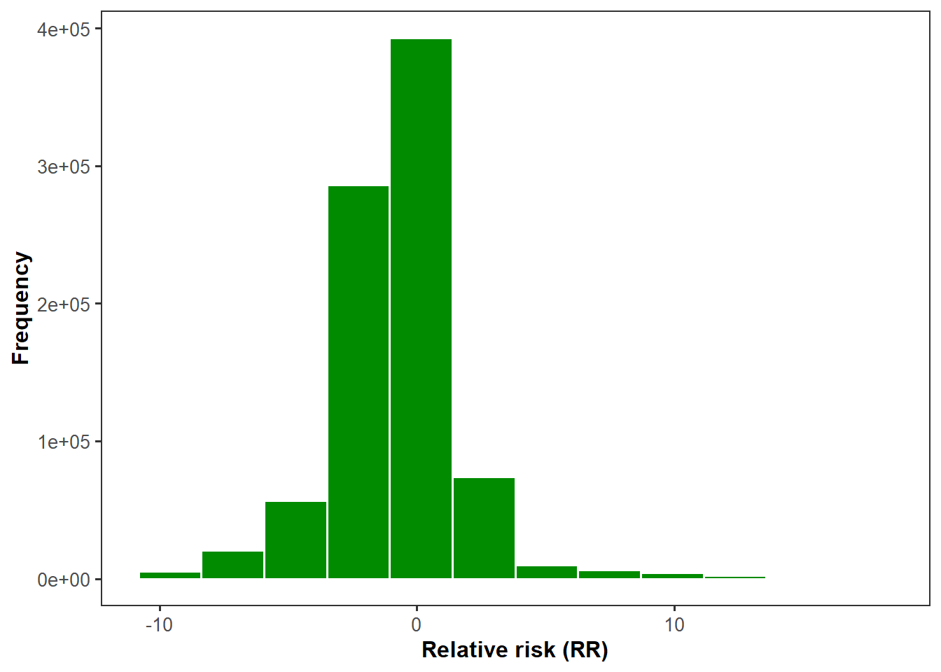

library(ggplot2)
library(dplyr)
library(scales)

lims <- quantile(df_heat$PERC, c(0.02, 0.98), na.rm = TRUE)
max_abs <- max(abs(lims))
df_plot <- df_heat %>%
  mutate(PERC_c = pmax(pmin(PERC,  max_abs), -max_abs))  


vpd_movel = df_plot %>% 
ggplot(aes(x = lag, y = tmean_val, fill = PERC_c)) +
  geom_raster(interpolate = TRUE) +
  geom_contour(aes(z = PERC), color = "black", size = 0.25,
               breaks = c(-15, -10, -5, 0, 5, 10, 15)) +
  geom_text_contour(aes(z = PERC), breaks = 0, stroke = 0.15,
                    label.padding = unit(0.15, "lines"), size = 3.2) +
scale_fill_gradient2(
  low = "#2c7bb6", mid = "white", high = "#d7191c",
  midpoint = 0, limits = c(-max_abs, max_abs),
  oob = squish,
  name = "RR (%)",
  guide = guide_colorbar(
    barwidth  = unit(4, "cm"),  
    barheight = unit(0.5, "cm") 
  )
) +
  scale_x_continuous(trans = "reverse",
    breaks = pretty(df_plot$lag, n = 8), expand = c(0, 0)) +
  scale_y_continuous(breaks = pretty(df_plot$tmean_val, n = 6), expand = c(0, 0)) +
  coord_cartesian(clip = "off") +
  labs(
    x = "Lag (days)",
    y = "VPD (kPa)") +
  theme_bw(base_size = 12) +
  theme(
    panel.grid = element_blank(),
    axis.title = element_text(face = "bold", size = 12),
    axis.text  = element_text(size = 10),
    legend.title = element_text(face = "bold"),
    plot.title = element_text(face = "bold", size = 13),
    plot.subtitle = element_text(size = 10),
    legend.position = "top"
  )

vpd_movel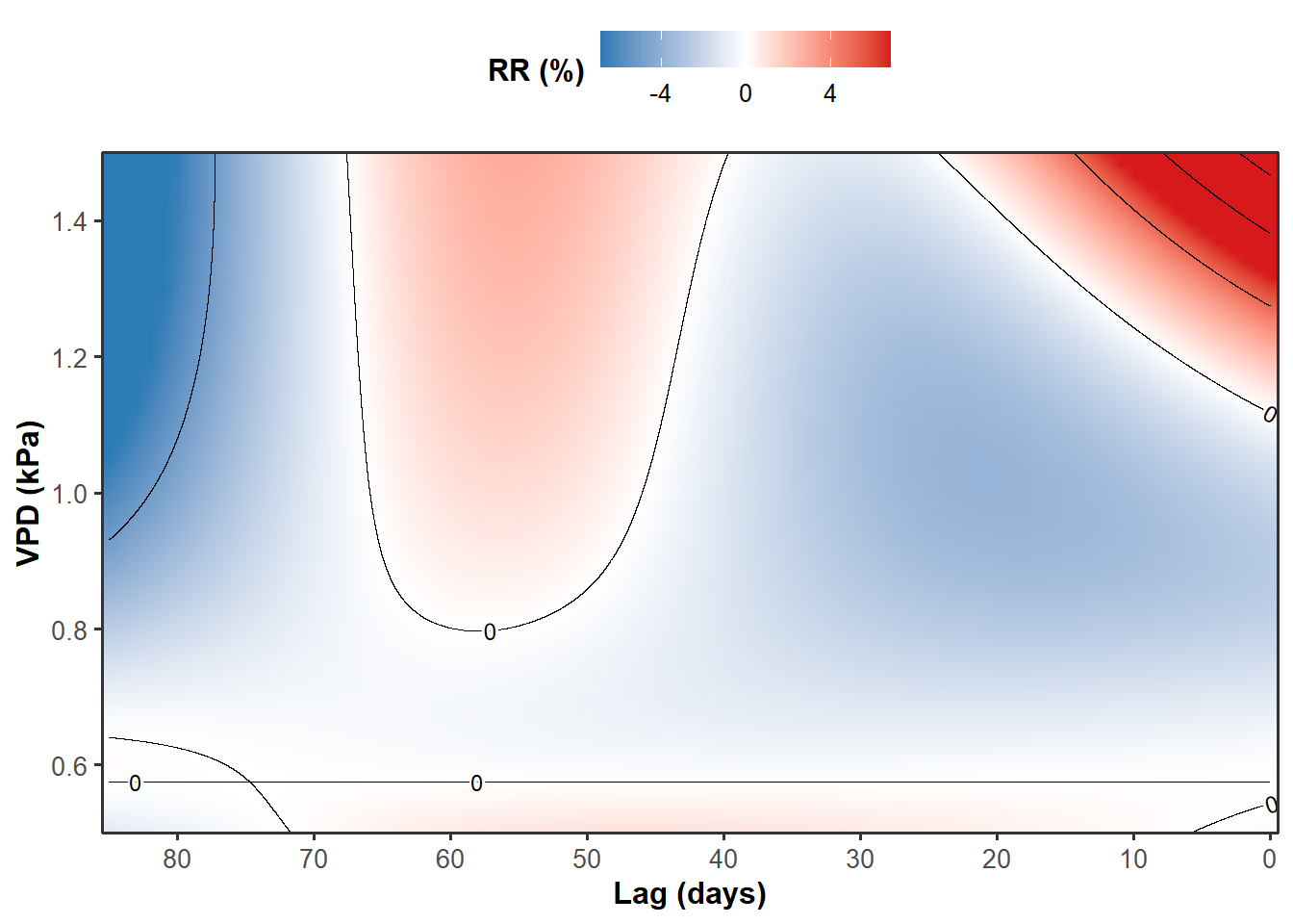

#tmean_movel/rain_movel/vpd_movel|sev_tmean/sev_rain/sev_vpd

(tmean_movel+rain_movel+vpd_movel)/(freq_tmax+freq_rain+freq_vpd)+
  plot_annotation(
    tag_levels = "a",
    tag_prefix = "(",
    tag_suffix = ")"
  ) &
  theme(
    plot.tag = element_text(face = "bold", size = 14),
    plot.tag.position = c(0, 1) 
  )

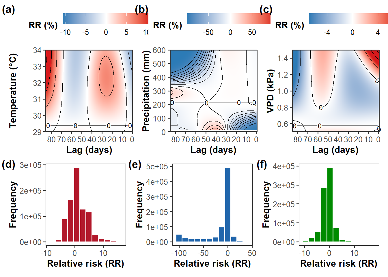
#ggsave("fig/RR_movel.png", dpi = 600, width = 10, height = 6)

Severity

suppressPackageStartupMessages({
  library(dplyr)
  library(dlnm)
  library(glmmTMB)
  library(ggplot2)
})

# ============================================================
# PREREQUISITES (must exist in the environment):
#   fit_sel      : fitted beta-logit glmmTMB model
#   dat          : data.frame used for fitting (with cb_* columns)
#   wx_use       : weather data (epi_id, tmax, rain_cum, vpd)
#   cb_templates : list with crossbasis templates (tmax, rain_cum, vpd)
#   LAG_MAX      : maximum lag (e.g., 85)
# ============================================================
stopifnot(exists("fit_sel"), exists("dat"), exists("wx_use"),
          exists("cb_templates"), exists("LAG_MAX"))

# ------------------------------------------------------------
# 1) UTILITIES
# ------------------------------------------------------------
get_cb_names <- function(dat, var) {
  grep(paste0("^cb_", var, "_"), names(dat), value = TRUE)
}

# typical time series length per epidemic
n_ref <- wx_use %>%
  filter(!is.na(vpd)) %>%
  count(epi_id) %>%
  pull(n) %>%
  median() %>%
  as.integer()

# ensure support for all lags
n_ref <- max(n_ref, LAG_MAX + 1)

# create a daily series with value "value" only within the lag band
make_series_band <- function(value, cen, n_ref, band = NULL) {
  x <- rep(cen, n_ref)
  if (!is.null(band)) {
    lags <- 0:(n_ref - 1)
    idx  <- which(lags %in% band)
    pos  <- n_ref - idx
    x[pos] <- value
  } else {
    x[] <- value
  }
  x
}

# extract the last row of the crossbasis
last_cb_row <- function(x, cb_template, LAG_MAX) {
  cbx <- dlnm::crossbasis(
    x, lag = LAG_MAX,
    argvar = attr(cb_template, "argvar"),
    arglag = attr(cb_template, "arglag")
  )
  as.numeric(cbx[length(x), ])
}

# manual prediction (population-level; beta-logit)
predict_eta_mu <- function(bt, br, bv, beta, nm_t, nm_r, nm_v) {
  eta <- unname(beta["(Intercept)"]) +
    sum(unname(beta[nm_t]) * bt) +
    sum(unname(beta[nm_r]) * br) +
    sum(unname(beta[nm_v]) * bv)
  mu <- plogis(eta)
  c(eta = eta, mu = mu)
}

# ------------------------------------------------------------
# 2) COLUMN NAMES cb_* IN THE MODEL
# ------------------------------------------------------------
nm_t <- get_cb_names(dat, "tmax")
nm_r <- get_cb_names(dat, "rain_cum")
nm_v <- get_cb_names(dat, "vpd")
stopifnot(length(nm_t) > 0, length(nm_r) > 0, length(nm_v) > 0)

# ------------------------------------------------------------
# 3) FIXED COEFFICIENTS
# ------------------------------------------------------------
beta <- fixef(fit_sel)$cond
stopifnot(all(c("(Intercept)", nm_t, nm_r, nm_v) %in% names(beta)))

# ------------------------------------------------------------
# 4) BASELINE (P50)
# ------------------------------------------------------------
cen_t <- as.numeric(quantile(wx_use$tmax,     0.50, na.rm = TRUE))
cen_r <- as.numeric(quantile(wx_use$rain_cum, 0.50, na.rm = TRUE))
cen_v <- as.numeric(quantile(wx_use$vpd,      0.50, na.rm = TRUE))

# baseline series
xt0 <- make_series_band(cen_t, cen_t, n_ref, band = NULL)
xr0 <- make_series_band(cen_r, cen_r, n_ref, band = NULL)
xv0 <- make_series_band(cen_v, cen_v, n_ref, band = NULL)

bt0 <- last_cb_row(xt0, cb_templates[["tmax"]],     LAG_MAX)
br0 <- last_cb_row(xr0, cb_templates[["rain_cum"]], LAG_MAX)
bv0 <- last_cb_row(xv0, cb_templates[["vpd"]],      LAG_MAX)

# baseline severity
base <- predict_eta_mu(bt0, br0, bv0, beta, nm_t, nm_r, nm_v)
sev_base_pct <- 100 * base["mu"]

# ------------------------------------------------------------
# 5) VPD GRID
# ------------------------------------------------------------
v_grid <- seq(0, 2.0, length.out = 200)

# periods
band_later   <- 0:40      # Later
band_earlier <- 41:85     # Earlier

# ------------------------------------------------------------
# 6) FUNCTION TO COMPUTE CURVES BY PERIOD
# ------------------------------------------------------------
calc_curve_phase_vpd <- function(values, band) {
  sapply(values, function(val) {

    xv <- make_series_band(
      value = val,
      cen   = cen_v,
      n_ref = n_ref,
      band  = band
    )

    bv <- last_cb_row(xv, cb_templates[["vpd"]], LAG_MAX)

    pr <- predict_eta_mu(bt0, br0, bv, beta, nm_t, nm_r, nm_v)

    100 * pr["mu"]
  })
}

# ------------------------------------------------------------
# 7) COMPUTE BOTH CURVES
# ------------------------------------------------------------
sev_vpd_later   <- calc_curve_phase_vpd(v_grid, band_later)
sev_vpd_earlier <- calc_curve_phase_vpd(v_grid, band_earlier)

df_vpd <- data.frame(
  vpd = rep(v_grid, 2),
  sev_pct = c(sev_vpd_earlier, sev_vpd_later),
  phase = rep(c("Earlier", "Later"), each = length(v_grid))
)

# ------------------------------------------------------------
# 8) PLOT — dashed vs solid
# ------------------------------------------------------------

sev_vpd = ggplot(df_vpd, aes(vpd, sev_pct, linetype = phase)) +
  #geom_hline(yintercept = 100*sev_base, linetype = 2, alpha = 0.6) +
  geom_smooth(method = "gam",
              formula = y ~ s(x, bs = "cs", k = 2),
              se = FALSE,
              linewidth = 2, colour = "green4")+
  #scale_color_brewer(palette = "Dark2") +
  labs(
    x = "VPD (kPa)",
    y = "Severity (%)",
    linetype = "Phases") +
  theme_bw(base_size = 12) +
  theme(
    legend.title = element_text(face = "bold"),
    axis.title = element_text(face = "bold", size = 12),
    axis.text  = element_text(size = 10))+
  scale_x_continuous(
    limits = c(0.5, 2),
    breaks = seq(0.5, 2, by = 0.25),
    expand = c(0, 0))+
   scale_y_continuous(
    limits = c(50, 100),
    breaks = seq(0, 100, by = 25),
    expand = c(0, 0))

sev_vpd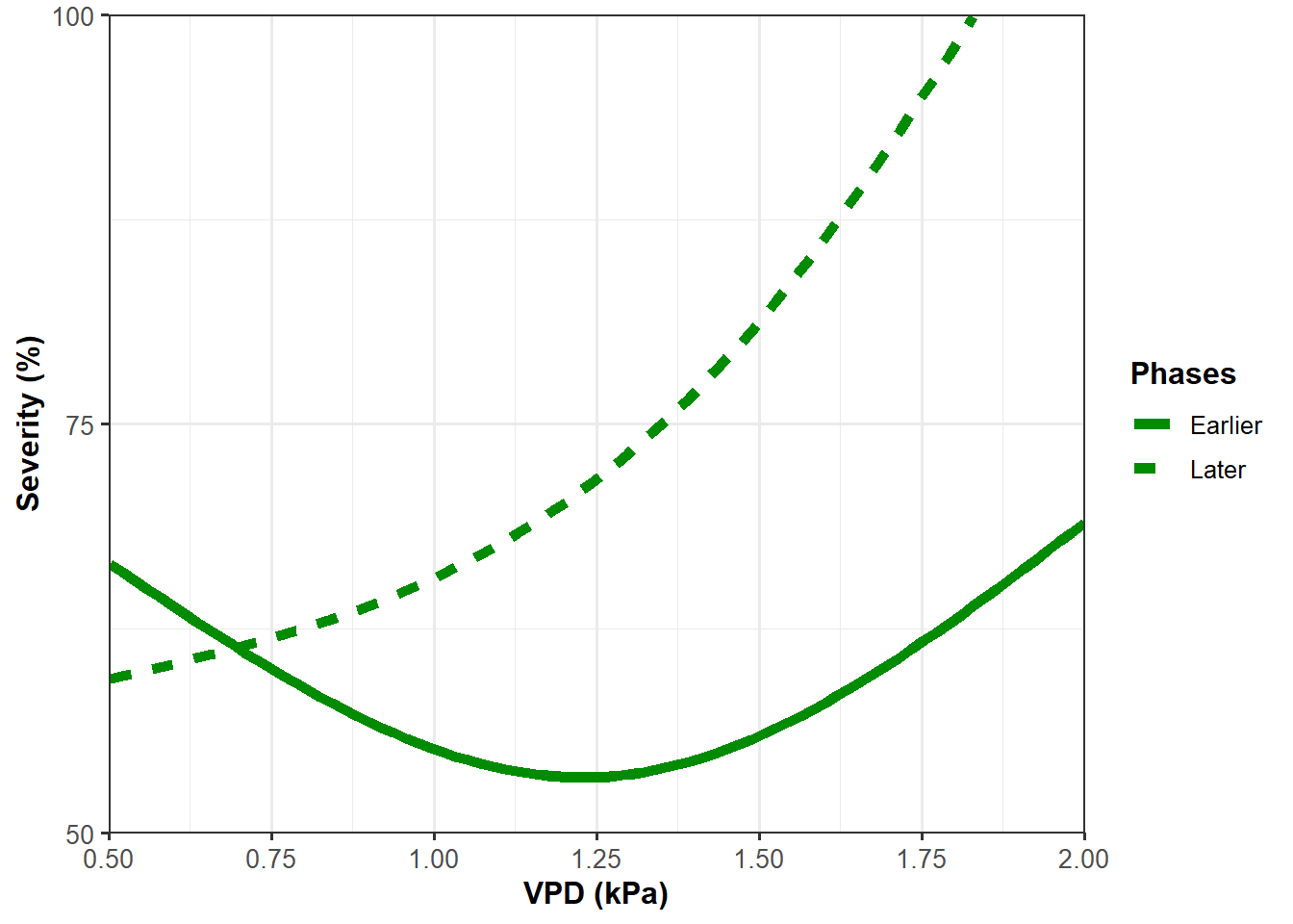

Delta

# ==============================================================
# DLNM heatmap / curves by lag bands (GLMMTMB beta-logit)
# - Effect of a single variable (e.g., tmax) across lags
# - BASELINE consistent with the DLNM "cen":
#     baseline = population-level prediction under the reference scenario:
#       tmax = P50(tmax), rain_cum = P50(rain_cum), vpd = P50(vpd)
# - Converts cumulative effect (Δη 0→L) into severity (%) via logit
# ==============================================================
# Expected inputs in the environment:
#   fit_sel      : glmmTMB beta_family(link="logit")
#   dat          : data.frame used for model fitting (contains cb_* columns)
#   cb_templates : list with crossbasis objects used in fitting (tmax, rain_cum, vpd)
#   wx_use       : data.frame/object with original time series containing epi_id and columns tmax, rain_cum, vpd
#   LAG_MAX      : maximum lag used in the crossbasis
# ==============================================================

suppressPackageStartupMessages({
  library(dlnm)
  library(glmmTMB)
  library(dplyr)
  library(tidyr)
  library(ggplot2)
  library(scales)
})

# --------------------- 0) Checks ---------------------------
stopifnot(exists("fit_sel"), exists("dat"), exists("cb_templates"),
          exists("wx_use"), exists("LAG_MAX"))

# --------------------- 1) Parameters --------------------------
var <- "vpd"   

if (is.null(cb_templates[[var]])) stop("cb_templates[['", var, "']] does not exist.")
if (!all(c("tmax","rain_cum","vpd") %in% names(cb_templates))) {
  stop("cb_templates must contain: 'tmax', 'rain_cum', 'vpd'.")
}

x_all <- wx_use[[var]]
if (is.null(x_all)) stop("wx_use[['", var, "']] does not exist.")

# DLNM "cen": P50 of the target variable
P50_var <- as.numeric(quantile(x_all, 0.50, na.rm = TRUE))

at_vals <- seq(0.50, 2.0, length.out = 1000)

# trim the range to the observed interval to avoid extrapolation
rng_obs <- range(x_all, na.rm = TRUE)
if (min(at_vals) < rng_obs[1] || max(at_vals) > rng_obs[2]) {
  message("WARNING: at_vals includes values outside the observed range: ",
          "observed range = [", round(rng_obs[1],2), ", ", round(rng_obs[2],2), "]")
}

# Lags for plotting
lag_max_plot <- 85L
lag_max_plot <- min(lag_max_plot, LAG_MAX)

# --------------------- 2) Coefs/VCOV only for cb_vpd block------------------
cb <- cb_templates[[var]]

cf_all <- coef(summary(fit_sel))$cond[, 1]
vc_all <- vcov(fit_sel)$cond

pref <- paste0("^cb_", var, "_")

idx_beta <- grep(pref, names(cf_all))
if (length(idx_beta) == 0) stop("Could not find cb_ coefficients for var='", var, "'.")
beta <- cf_all[idx_beta]

idx_rows <- grep(pref, rownames(vc_all))
idx_cols <- grep(pref, colnames(vc_all))
V <- vc_all[idx_rows, idx_cols, drop = FALSE]

# Checagens
if (length(beta) != ncol(cb)) stop("length(beta) != ncol(cb). check cb_templates and model.")
if (!(nrow(V) == ncol(cb) && ncol(V) == ncol(cb))) stop("VCOV does not match ncol(cb).")

# --------------------- 3) crosspred: Δη by lag vs cen=P50_var ----------------
cp <- dlnm::crosspred(
  cb,
  coef  = beta,
  vcov  = V,
  at    = at_vals,
  cen   = P50_var,
  bylag = 1
)

mf <- cp$matfit  # Δη (link) by lag; rows=at_vals, columns=lags

# Sort lags
lag_idx <- suppressWarnings(as.integer(gsub("lag", "", colnames(mf))))
if (anyNA(lag_idx)) {
  lag_idx <- 0:(ncol(mf) - 1)
  colnames(mf) <- paste0("lag", lag_idx)
}
ord <- order(lag_idx)
mf <- mf[, ord, drop = FALSE]
lag_idx <- lag_idx[ord]

# keep 0..lag_max_plot
keep <- which(lag_idx >= 0 & lag_idx <= lag_max_plot)
mf <- mf[, keep, drop = FALSE]
lag_idx <- lag_idx[keep]

# --------------------- 4) Consistent baseline (joint P50 scenario) ------------
# References (P50) for ALL model variables
P50_t <- as.numeric(quantile(wx_use[["tmax"]],     0.50, na.rm = TRUE))
P50_r <- as.numeric(quantile(wx_use[["rain_cum"]], 0.50, na.rm = TRUE))
P50_v <- as.numeric(quantile(wx_use[["vpd"]],      0.50, na.rm = TRUE))

# n_ref (typical series length)
n_ref <- wx_use %>%
  filter(!is.na(tmax)) %>%
  count(epi_id) %>%
  pull(n) %>%
  stats::median() %>%
  as.integer()

n_ref <- max(n_ref, LAG_MAX + 1)

# cb_* names in dat
nm_t <- grep("^cb_tmax_",     names(dat), value = TRUE)
nm_r <- grep("^cb_rain_cum_", names(dat), value = TRUE)
nm_v <- grep("^cb_vpd_",      names(dat), value = TRUE)
stopifnot(length(nm_t) > 0, length(nm_r) > 0, length(nm_v) > 0)

# function: last crossbasis row for constant series
last_cb_row_const <- function(value, cb_template, LAG_MAX, n_ref) {
  x <- rep(value, n_ref)
  cbx <- dlnm::crossbasis(
    x, lag = LAG_MAX,
    argvar = attr(cb_template, "argvar"),
    arglag = attr(cb_template, "arglag")
  )
  as.numeric(cbx[n_ref, ])
}

bt0 <- last_cb_row_const(P50_t, cb_templates[["tmax"]],     LAG_MAX, n_ref)
br0 <- last_cb_row_const(P50_r, cb_templates[["rain_cum"]], LAG_MAX, n_ref)
bv0 <- last_cb_row_const(P50_v, cb_templates[["vpd"]],      LAG_MAX, n_ref)

# reference newdata
nd0 <- data.frame(siteyear = dat$siteyear[1])
nd0[nm_t] <- as.list(bt0)
nd0[nm_r] <- as.list(br0)
nd0[nm_v] <- as.list(bv0)

# baseline pop-level (random effects set to zero)
sev_base <- as.numeric(predict(fit_sel, newdata = nd0, type = "response", re.form = NA))

# --------------------- 5) Convert cumulative Δη 0→L into final severity -----
mf_cum <- t(apply(mf, 1, cumsum))

SEV_mat <- plogis(qlogis(sev_base) + mf_cum)         # 0–1
SEVdiff_pp <- 100 * (SEV_mat - sev_base)             # percentage point (pp)

# --------------------- 6) Data frame long (heatmap Δpp) -----------------------
df_diff <- as.data.frame(SEVdiff_pp)
colnames(df_diff) <- paste0("lag_", lag_idx)

df_diff <- df_diff %>%
  mutate(var_val = at_vals) %>%
  pivot_longer(starts_with("lag_"), names_to = "lag", values_to = "SEV_diff_pp") %>%
  mutate(lag = as.integer(gsub("lag_", "", lag)))

# --------------------- 7) Heatmap (Δ in pp) ----------------------------------
p_heat_diff_vpd <- ggplot(df_diff, aes(x = lag, y = var_val, fill = SEV_diff_pp)) +
  geom_raster() +
  scale_fill_viridis_c(name = "Δ (pp)") +
  labs(
    x = "Lag (days)",
    y = "VPD (kPa)") +
  theme_bw(base_size = 12) +
  theme(plot.title = element_text(face = "bold"),
        axis.title = element_text(face = "bold"))+
  scale_x_continuous(
    trans = "reverse",
    breaks = c(0,10,20,30,40,50,60,70,80),
    limits = c(0,85),
    expand = c(0, 0)
  ) +
  scale_y_continuous(
    limits = c(0.5, 2),
    breaks = seq(0.5, 2, by = 0.25),
    expand = c(0, 0))

print(p_heat_diff_vpd)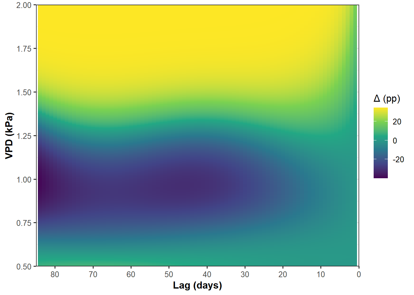

((p_heat_diff_tmax/p_heat_diff_rain/p_heat_diff_vpd)|(sev_tmax/sev_rain/sev_vpd))+
  plot_annotation(
    tag_levels = "a",
    tag_prefix = "(",
    tag_suffix = ")"
  ) &
  theme(
    plot.tag = element_text(face = "bold", size = 14),
    plot.tag.position = c(0, 1) 
  )

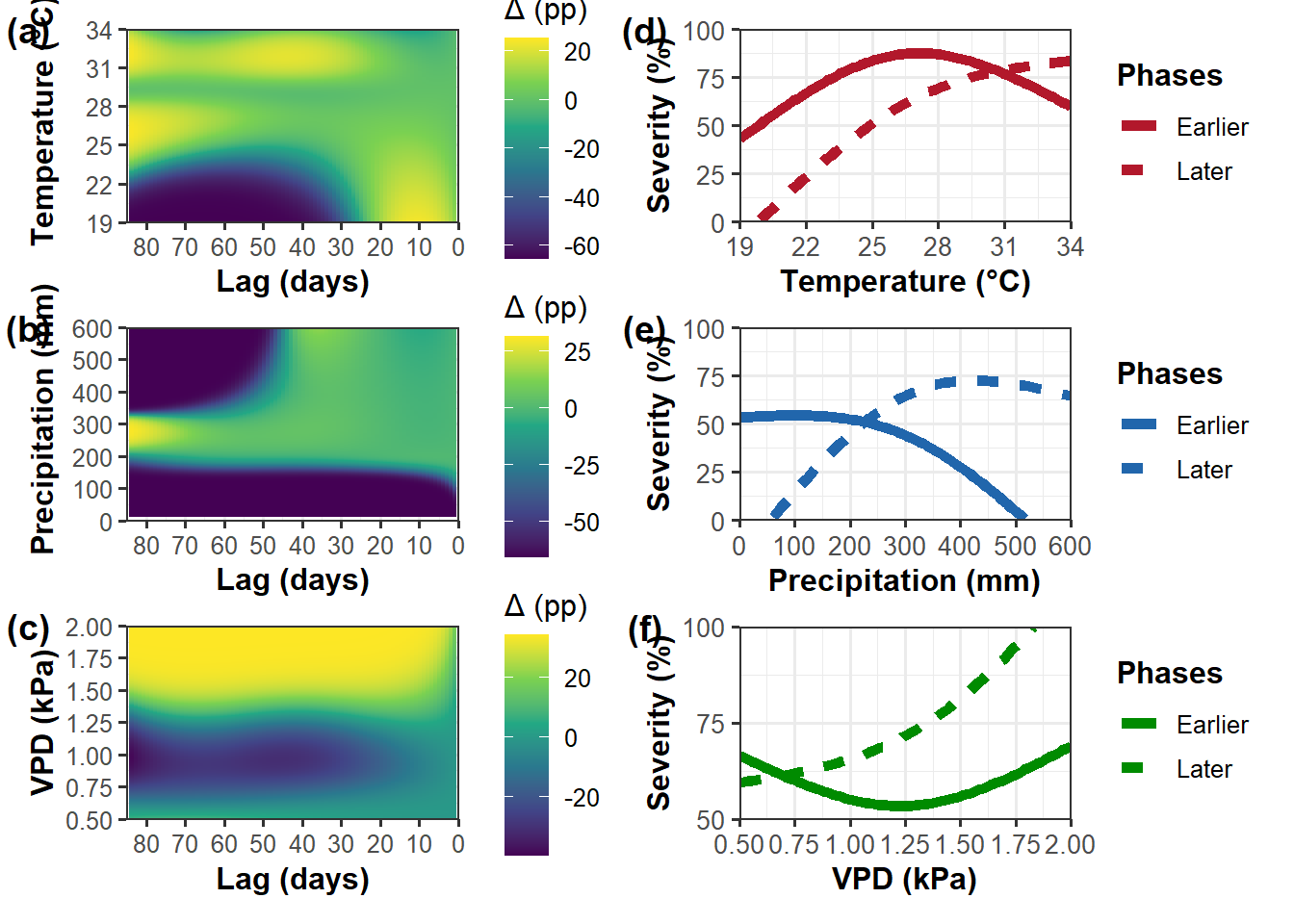
#ggsave("fig/delta_severity.png", dpi = 600, width = 10, height = 8)

Discriptive plotting

wx_use2 = read_xlsx("data/ERA5_weather2.xlsx")

wx_use2 = wx_use2 %>% 
  left_join(epi_use, by = "epi_id")

wx_use2 %>% 
  group_by(year.x,state.x) %>% 
  summarise(
    mean = mean(sev)
  ) %>% 
  filter(state.x == "TO")

wx_use2$year.x = wx_use2$year.x-1

wx_use2 <- wx_use2 %>%
  mutate(
    year = paste0(year.x, "/", year.x + 1)
  )

vpd_state = wx_use2 %>% 
  ggplot(aes(dpp,vpd, group = as.factor(year), color = as.factor(year)))+
  geom_smooth(se = F)+
  facet_wrap(~state.x, ncol = 3)+
  theme_bw()+
  scale_color_viridis_d()+
  theme(
    text = element_text(size = 14),
    axis.title = element_text(face = "bold"),
    legend.position = "right",
    strip.background = element_blank(),
    strip.text = element_text(size = 14, face = "bold")
  )+
  labs(x = "DPP",
       y = "VPD (kPa)",
       color = "")

vpd_state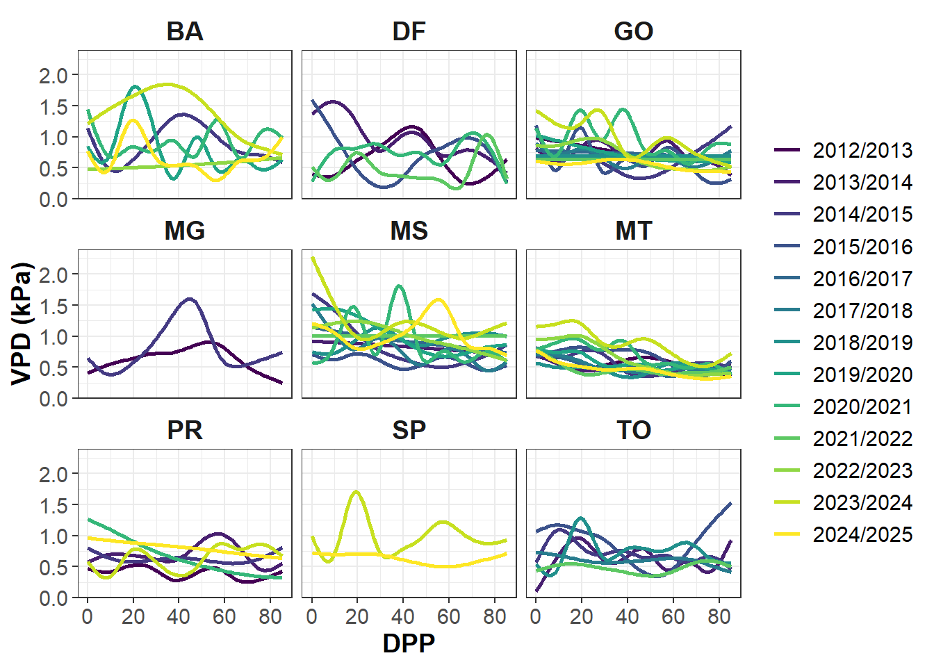

ggsave("fig/vpd_state.png", dpi = 600, width = 14, height = 10)

tmax_state = wx_use2 %>% 
  ggplot(aes(dpp,tmax, group = as.factor(year), color = as.factor(year)))+
  geom_smooth(se = F)+
  facet_wrap(~state.x, ncol = 3)+
  theme_bw()+
  scale_color_viridis_d()+
  theme(
    text = element_text(size = 14),
    axis.title = element_text(face = "bold"),
    legend.position = "right",
    strip.background = element_blank(),
    strip.text = element_text(size = 14, face = "bold")
  )+
  labs(x = "DPP",
       y = "Temperature (°C)",
       color = "")

tmax_state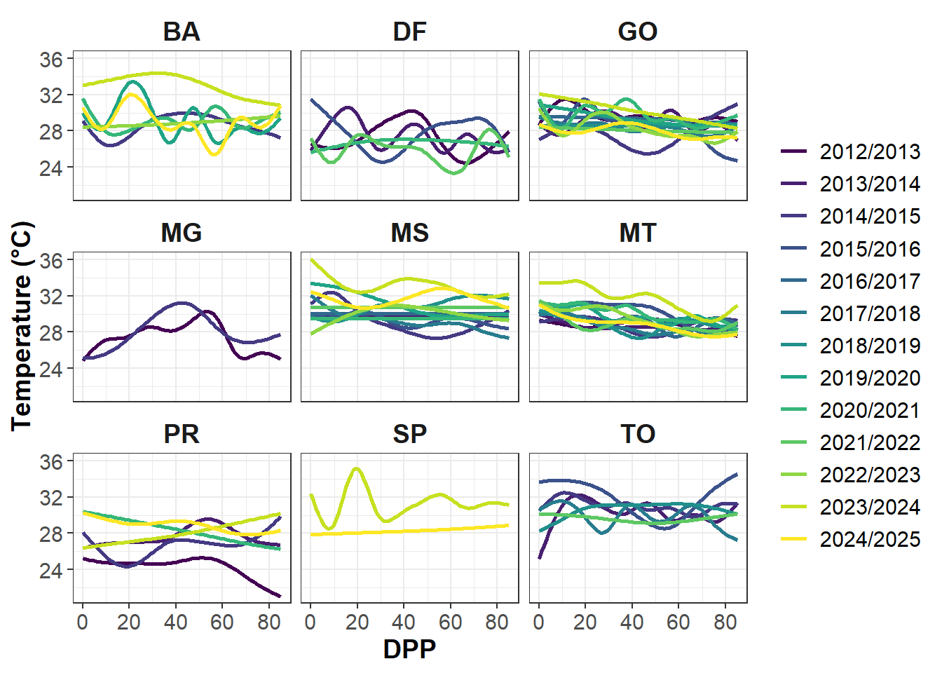

ggsave("fig/tmax_state.png", dpi = 600, width = 14, height = 10)

rain_state = wx_use2 %>% 
  ggplot(aes(dpp,rain_cum, group = as.factor(year), color = as.factor(year)))+
  geom_smooth(se = F)+
  facet_wrap(~state.x, ncol = 3)+
  theme_bw()+
  scale_color_viridis_d()+
    theme(
    text = element_text(size = 14),
    axis.title = element_text(face = "bold"),
    legend.position = "right",
    strip.background = element_blank(),
    strip.text = element_text(size = 14, face = "bold")
  )+
  labs(x = "DPP",
       y = "Precipitation (mm)",
       color = "")
rain_state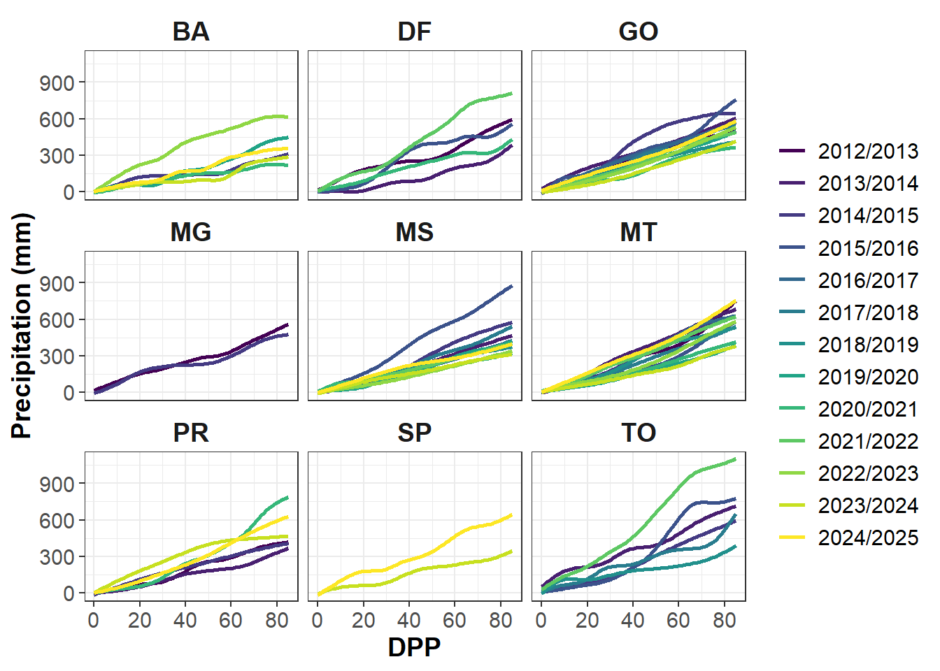

ggsave("fig/rain_state.png", dpi = 600, width = 14, height = 10)

Map

map = epi_use %>% 
  dplyr::select(study,year,location,state,latitude,longitude,sev)

colnames(map) = c("study","year","location","state","lat","lon","mean_sev")

library(scales)
library(ggspatial) 
library(readxl)
library(ggrepel)
library(cowplot)
library(rnaturalearth)

BRA = ne_states(
  country = "Brazil",
  returnclass = "sf"
)



states <- filter(BRA, 
                 name_pt == "Paraná"|
                 name_pt == "São Paulo"|
                 name_pt == "Mato Grosso"|
                 name_pt == "Mato Grosso do Sul"|
                 name_pt == "Goiás"|
                 name_pt == "Minas Gerais"|
                 name_pt == "Distrito Federal"|
                 name_pt == "Tocantins"|
                 name_pt == "Bahia")

states = states %>% 
  mutate(id = case_when(
    name_pt == "Paraná" ~ "PR",
    name_pt == "São Paulo" ~ "SP",
    name_pt == "Mato Grosso" ~ "MT",
    name_pt == "Mato Grosso do Sul" ~ "MS",
    name_pt == "Goiás" ~ "GO",
    name_pt == "Minas Gerais" ~ "MG",
    name_pt == "Distrito Federal" ~ "DF",
    name_pt == "Tocantins" ~ "TO",
    name_pt == "Bahia" ~ "BA"))

SUL = ne_states(
  country = c("Argentina", "Uruguay", "Paraguay", "Colombia", "Bolivia"),
  returnclass = "sf")
br_sf <- ne_states(geounit = "brazil",
                   returnclass = "sf")

unique(map$state)

[1] "MT" "MS" "GO" "PR" "TO" "DF" "BA" "MG" "SP"

map_plot = map %>% 
ggplot()+
  geom_sf(data = SUL, fill = "gray95", color = "gray95") +
  geom_sf(data = BRA, fill = "gray98", color= "gray60", size =0.2) +
  geom_sf(data = states, aes(x = longitude, y = latitude), fill = "white", color = "gray40", size = 0.2) +
  geom_jitter(data = map, aes(as.numeric(lon), as.numeric(lat)), size = 4, alpha = 0.8, color = "#002f61") +
  geom_text(data = states, aes(x = longitude, y = latitude,  label = id), size = 3, hjust = 0.8, fontface = "bold")+
  labs(x = "Longitude", y = "Latitude", color = "Region", size = "Number of Trials") +
  scale_size_continuous(range = c(1,5), breaks = c(1,5,12))+
  #theme_bw()+
  theme_minimal_grid()+
  annotation_scale(location = "bl", width_hint = 0.2) +
  coord_sf(xlim = c(-65,-40), ylim = c(-32, -9), expand = FALSE)+
  #scale_color_calc()+
  theme(legend.position = "right",
        legend.justification = "center",
        legend.title.align = 0.5,
        legend.title = element_text(size = 10, face = "bold"),
        legend.text = element_text(size = 10),
        axis.text.x =  element_text(size = 9),
        axis.text.y = element_text(size = 9),
        axis.title.x = element_text(size=12, face = "bold"),
        axis.title.y = element_text(size=12, face = "bold"),
        panel.border = element_rect(color = "gray50", size=.2),
        panel.background = element_rect(fill = "#d2eeff")
        )+
  annotation_north_arrow(location = "bl", which_north = "true", pad_x = unit(0.5, "in"), pad_y = unit(0.5, "in"), style = north_arrow_orienteering(fill = c("gray80", "gray96")), height = unit(0.9, "cm"), width = unit(0.8, "cm"))+
  guides(size=F)

map_plot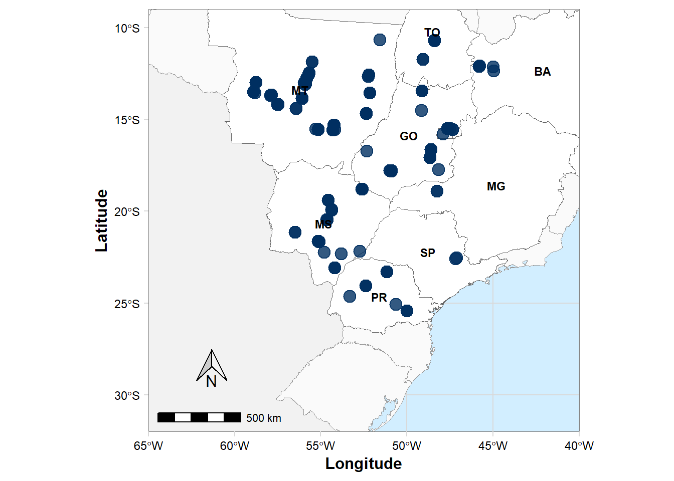

sev_plot = map %>% 
  ggplot(aes(mean_sev))+
  geom_histogram(fill = "#002f61", color = "white", bins = 15)+
  ggthemes::theme_few()+
  labs(x = "Severity (%)",
       y = "Frequency")+
  theme(text = element_text(size = 12),
        axis.title = element_text(face = "bold"),
        axis.text.x = element_text(angle = 45, vjust = 0.5))

map <- map %>%
  mutate(
    year = year - 1
  ) %>% 
  mutate(
    year = paste0(year, "/", year + 1)
  )

year_plot= map %>% 
dplyr::group_by(year) %>% 
  summarise(
   mean_sev = mean(mean_sev)
  ) %>% 
  ggplot(aes(as.factor(year),mean_sev))+
  geom_bar(stat = "identity" ,fill = "#002f61")+
  ggthemes::theme_few()+
  labs(x = "Season",
       y = "Severity (%)")+
  theme(text = element_text(size = 12),
        axis.title = element_text(face = "bold"),
        axis.text.x = element_text(angle = 45, vjust = 1, hjust = 0.9))

year_plot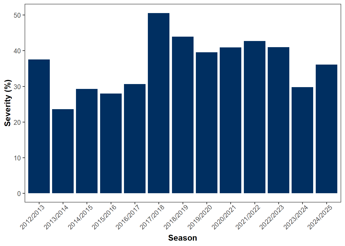

(map_plot + (sev_plot / year_plot)) + 
  plot_layout(design = "AB
                        AB", widths = c(2, 1)) +
  plot_annotation(tag_levels = "a", tag_prefix = "(", tag_suffix = ")") & 
  theme(plot.tag = element_text(face = "bold", size = 12), label_x = -0.03, label_y = 1)


ggsave("fig/map_sev_year2.png", dpi = 600, bg = "white",
       width = 12, height = 8)

Scenarios simulation (Severity)

suppressPackageStartupMessages({
  library(dplyr)
  library(tidyr)
  library(purrr)
  library(dlnm)
  library(glmmTMB)
  library(ggplot2)
})

# =========================
# PRE-REQUISITES
# =========================
stopifnot(exists("fit_sel"), exists("dat"), exists("wx_use"), exists("cb_templates"), exists("LAG_MAX"))

# -------------------------
# periods (lags)
# -------------------------
LAG_BAND_LATER   <- 0:40          # Later
LAG_BAND_EARLIER <- 41:LAG_MAX    # Earlier
N <- LAG_MAX + 1

# -------------------------
# Baseline (P50) — used as a reference (not to replace your scenarios)
# -------------------------
base_vals <- list(
  tmax     = as.numeric(quantile(wx_use$tmax,     0.50, na.rm = TRUE)),
  rain_cum = as.numeric(quantile(wx_use$rain_cum, 0.50, na.rm = TRUE)),
  vpd      = as.numeric(quantile(wx_use$vpd,      0.50, na.rm = TRUE))
)

# -------------------------
# Auxiliary functions (scenarios by periods)
# -------------------------
lags_to_idx <- function(N, lags) {
  idx <- N - lags
  idx[idx >= 1 & idx <= N]
}

make_profile_two_windows <- function(N, base_value,
                                     lags_A, value_A,
                                     lags_B, value_B) {
  x <- rep(base_value, N)
  x[lags_to_idx(N, lags_A)] <- value_A
  x[lags_to_idx(N, lags_B)] <- value_B
  x
}

extract_last_cb_row <- function(x, cb_template) {
  cb <- dlnm::crossbasis(
    x, lag = LAG_MAX,
    argvar = attr(cb_template, "argvar"),
    arglag = attr(cb_template, "arglag")
  )
  as.numeric(cb[length(x), ])
}

get_cb_colnames <- function(dat, var) {
  grep(paste0("^cb_", var, "_"), names(dat), value = TRUE)
}

build_newdata_from_profiles <- function(dat, cb_templates, profiles, siteyear_level = NULL) {
  if (is.null(siteyear_level)) siteyear_level <- dat$siteyear[1]
  nd <- data.frame(siteyear = siteyear_level)

  for (v in names(profiles)) {
    cb_row <- extract_last_cb_row(profiles[[v]], cb_templates[[v]])
    cols   <- get_cb_colnames(dat, v)
    stopifnot(length(cb_row) == length(cols))
    nd[cols] <- as.list(cb_row)
  }
  nd
}

predict_two_window_scenario <- function(fit_sel, dat, cb_templates,
                                        base_vals, scen_later, scen_earlier,
                                        lags_later = LAG_BAND_LATER,
                                        lags_earlier = LAG_BAND_EARLIER,
                                        N = LAG_MAX + 1,
                                        pop_level = TRUE,
                                        siteyear_level = NULL) {

  profiles <- list(
    tmax = make_profile_two_windows(
      N, base_vals$tmax,
      lags_later,   scen_later$tmax,
      lags_earlier, scen_earlier$tmax
    ),
    rain_cum = make_profile_two_windows(
      N, base_vals$rain_cum,
      lags_later,   scen_later$rain_cum,
      lags_earlier, scen_earlier$rain_cum
    ),
    vpd = make_profile_two_windows(
      N, base_vals$vpd,
      lags_later,   scen_later$vpd,
      lags_earlier, scen_earlier$vpd
    )
  )

  nd <- build_newdata_from_profiles(dat, cb_templates, profiles, siteyear_level)

  if (pop_level) {
    pred <- predict(fit_sel, newdata = nd, type = "response", re.form = NA)
  } else {
    pred <- predict(fit_sel, newdata = nd, type = "response")
  }

  as.numeric(pred) # return (0,1)
}

# =========================
# Scenarios definition
# =========================
# rain per period:
# HH: earlier=400 later=400
# HB: earlier=400 later=100
# BH: earlier=100 later=400
# BB: earlier=100 later=100

rain_scenarios <- tibble::tribble(
  ~scenario, ~rain_earlier, ~rain_later,
  "HH",      350,           350,
  "HL",      350,           150,
  "LH",      150,           350,
  "LL",      150,           150
) %>%
  mutate(scenario = factor(scenario, levels = c("HH","HL","LH","LL")))

# VPD levels (lines inside the plot)
vpd_levels <- tibble::tribble(
  ~vpd_level, ~vpd_value,
  "Low",      0.6,
  "Medium",   1.1,
  "High",     1.5
) %>%
  mutate(vpd_level = factor(vpd_level, levels = c("Low","Medium","High")))

# temperature grid
t_grid <- seq(19, 34, length.out = 800)

# =========================
# SEVERITY BASELINE (P50/P50/P50)
# =========================
sev_base <- predict_two_window_scenario(
  fit_sel, dat, cb_templates,
  base_vals = base_vals,
  scen_later   = list(tmax=base_vals$tmax, rain_cum=base_vals$rain_cum, vpd=base_vals$vpd),
  scen_earlier = list(tmax=base_vals$tmax, rain_cum=base_vals$rain_cum, vpd=base_vals$vpd),
  pop_level = TRUE
)
sev_base_pct <- 100 * sev_base

# =========================
# GENERATE THE PREDICTION GRID
# =========================
pred_df <- expand.grid(
  scenario = levels(rain_scenarios$scenario),
  vpd_level = levels(vpd_levels$vpd_level),
  tmax = t_grid,
  KEEP.OUT.ATTRS = FALSE,
  stringsAsFactors = FALSE
) %>%
  as_tibble() %>%
  left_join(rain_scenarios, by = "scenario") %>%
  left_join(vpd_levels, by = "vpd_level") %>%
  mutate(
    scenario = factor(scenario, levels = c("HH","HL","LH","LL")),
    vpd_level = factor(vpd_level, levels = c("Low","Medium","High"))
  )

# function to predict 1 row
predict_row <- function(tmax_val, rain_earlier, rain_later, vpd_val) {

  scen_later <- list(
    tmax     = tmax_val,     # tmax applied to the side period
    rain_cum = rain_later,
    vpd      = vpd_val
  )

  scen_earlier <- list(
    tmax     = tmax_val,     # tmax applied in the Earlier period (same value)
    rain_cum = rain_earlier,
    vpd      = vpd_val       # vpd also constant in both period
  )

  100 * predict_two_window_scenario(
    fit_sel, dat, cb_templates,
    base_vals = base_vals,
    scen_later = scen_later,
    scen_earlier = scen_earlier,
    pop_level = TRUE
  )
}

# apply prediction to all combinations.
pred_df$sev_pct <- purrr::pmap_dbl(
  list(pred_df$tmax, pred_df$rain_earlier, pred_df$rain_later, pred_df$vpd_value),
  predict_row
)

#writexl::write_xlsx(pred_df,"data/pred_df.xlsx")

p <- pred_df %>%
  filter(!vpd_level == "Low") %>% 
  ggplot(aes(x = tmax, y = sev_pct, color = vpd_level)) +
geom_smooth(method = "gam",
              formula = y ~ s(x, bs = "cs", k = 2),
              se = FALSE,
              linewidth = 2) +

  facet_wrap(~ scenario, ncol = 2) +
  scale_color_manual(
    values = c("Low" = "#1b9e77", "Medium" = "green4", "High" = "#B2182B"),
    name = "VPD level") +
  labs(
    x = "Temperature (°C)",
    y = "Severity (%)") +
  theme_bw(base_size = 12) +
  theme(
    axis.title = element_text(face = "bold"),
    plot.title = element_text(face = "bold"),
    strip.text = element_text(face = "bold"),
    legend.title = element_text(face = "bold"),
    strip.background = element_blank())+
  coord_cartesian(ylim = c(0, 100))+
  scale_x_continuous(
    limits = c(19, 34),
    breaks = seq(19, 34, by = 3),
    expand = c(0.02, 0.02))

print(p)

#ggsave("fig/severity_scenarios.png", dpi = 600, width = 8, height = 6)

weather_data <- epi %>%
  mutate(
    # Creating the allowed date directly based on the state
    allowed_date = case_when(
      state == "MT" ~ as.Date(paste0(format(planting_date, "%Y"), "-09-16")), 
      state == "MS" ~ as.Date(paste0(format(planting_date, "%Y"), "-09-16")),
      state == "GO" ~ as.Date(paste0(format(planting_date, "%Y"), "-09-25")),
      state == "PR" ~ as.Date(paste0(format(planting_date, "%Y"), "-09-11")),
      state == "TO" ~ as.Date(paste0(format(planting_date, "%Y"), "-10-01")),
      state == "DF" ~ as.Date(paste0(format(planting_date, "%Y"), "-10-01")),
      state == "BA" ~ as.Date(paste0(format(planting_date, "%Y"), "-10-01")),
      state == "MG" ~ as.Date(paste0(format(planting_date, "%Y"), "-10-01")) 
    ),
    # Adjusting the allowed_date year for January and February cases.
    allowed_date = if_else(
      format(planting_date, "%m") %in% c("01", "02"), 
      as.Date(paste0(as.numeric(format(planting_date, "%Y")) - 1, "-", format(allowed_date, "%m-%d"))),
      allowed_date
    ),
    # Calculating the difference in days
    days_difference = as.numeric(planting_date - allowed_date)
  )

ERA5 map

Early

points = read_xlsx("data/points_states.xlsx")

#years <- 2012:2024
years <- 2005:2024

p_states <- crossing(points, year = years)


p_states <- p_states %>%
  mutate(
    # Creating the allowed date directly based on the state
    allowed_date = case_when(
      state == "MT" ~ as.Date(paste0(format(year), "-09-16")), 
      state == "MS" ~ as.Date(paste0(format(year), "-09-16")),
      state == "GO" ~ as.Date(paste0(format(year), "-09-25")),
      state == "PR" ~ as.Date(paste0(format(year), "-09-11")),
      state == "TO" ~ as.Date(paste0(format(year), "-10-01")),
      state == "DF" ~ as.Date(paste0(format(year), "-10-01")),
      state == "BA" ~ as.Date(paste0(format(year), "-10-01")),
      state == "MG" ~ as.Date(paste0(format(year), "-10-01")) ,
      state == "SP" ~ as.Date(paste0(format(year), "-10-01")) 
    ))


p_states$id1 <- seq_len(nrow(p_states))


p_states <- p_states %>%
  mutate(
    id1 = as.integer(id1),
    allowed_date = as.Date(allowed_date)
  )

#p_states = p_states %>% 
 # mutate(
  #  PD85 = allowed_date+85
  #)


p_states <- p_states %>%
  mutate(PD85 = allowed_date + 85) 

max(p_states$PD85)

[1] "2024-12-25"

cutoff_date <- as.Date("2024-12-25")

p_states <- p_states %>%
  filter(PD85 <= cutoff_date)

unique(p_states$year)

 [1] 2005 2006 2007 2008 2009 2010 2011 2012 2013 2014 2015 2016 2017 2018 2019
[16] 2020 2021 2022 2023 2024

min(p_states$allowed_date)

[1] "2005-09-11"

max(p_states$allowed_date)

[1] "2024-10-01"

max(p_states$PD85)

[1] "2024-12-25"

TMAX

library(terra)
library(data.table)
library(lubridate)

#nc_path <- "/media/amazonia/hd2/lais/Ricardo/DLNM/data/data/era5land_daily_tmax_2012_2025.nc"
nc_path <- "/media/amazonia/hd2/lais/Ricardo/DLNM/data/data/era5land_daily_tmax_2005_2025.nc"
out_dir <- "/media/amazonia/hd2/lais/Ricardo/DLNM/data/output_tmax_yearly"

dir.create(out_dir, recursive = TRUE, showWarnings = FALSE)

# RAM
chunk_size <- 5000

# =========================================================
# 2) PREPARE p_states
# =========================================================
p_states_dt <- as.data.table(p_states)

p_states_dt[, allowed_date := as.Date(allowed_date)]
p_states_dt[, PD85         := as.Date(PD85)]
p_states_dt[, pt_id        := .I]
p_states_dt[, year_allowed := year(allowed_date)]

# keep only valid lines
p_states_dt <- p_states_dt[
  !is.na(longitude) & !is.na(latitude) &
  !is.na(allowed_date) & !is.na(PD85)
]

# ensure a maximum period of 85 days
p_states_dt[PD85 > allowed_date + 85, PD85 := allowed_date + 85]

# =========================================================
# 3) READ NetCDF ONCE
# =========================================================
r <- rast(nc_path)

dates_all <- as.Date(time(r))
if (all(is.na(dates_all))) {
  stop("Datas não encontradas no NetCDF.")
}

layer_names <- names(r)

# Raster CRS
r_crs <- crs(r)

# =========================================================
# 4) FUNCTION TO PROCESS ONE YEAR
# =========================================================
process_year <- function(yr, pts_year, r, dates_all, layer_names,
                         out_dir, chunk_size = 5000) {

  cat("\n=============================\n")
  cat("Processing year:", yr, "\n")
  cat("N points:", nrow(pts_year), "\n")

  # minimum interval required for this year
  date_ini <- min(pts_year$allowed_date, na.rm = TRUE)
  date_fim <- max(pts_year$PD85, na.rm = TRUE)

  cat("necessary interval:", as.character(date_ini), "until", as.character(date_fim), "\n")

  # strictly necessary raster layers
  idx <- which(dates_all >= date_ini & dates_all <= date_fim)

  if (length(idx) == 0) {
    cat("No layers found for this range. Skipping.\n")
    return(NULL)
  }

  r_sub <- r[[idx]]
  dates_sub <- dates_all[idx]
  layer_names_sub <- layer_names[idx]

  cat("N used layers:", length(idx), "\n")

  # output (year)
  out_file <- file.path(out_dir, paste0("tmax_window_", yr, ".csv.gz"))

  # Remove if it already exists.
  if (file.exists(out_file)) file.remove(out_file)

  n <- nrow(pts_year)
  starts <- seq(1, n, by = chunk_size)

  for (s in starts) {
    e <- min(s + chunk_size - 1, n)
    cat("  Chunk:", s, "-", e, "de", n, "\n")

    pts_chunk <- pts_year[s:e]

    # Create spatial vector
    pts_v <- vect(
      pts_chunk,
      geom = c("longitude", "latitude"),
      crs  = "EPSG:4326"
    )

    # redesign if necessary
    if (!is.na(r_crs) && r_crs != crs(pts_v)) {
      pts_v <- project(pts_v, r_crs)
    }

    # extraction
    ext <- terra::extract(
      r_sub,
      pts_v,
      xy = TRUE,
      ID = FALSE
    )

    ext_dt <- as.data.table(ext)

    # Add pt_id in the same order as the chunk
    ext_dt[, pt_id := pts_chunk$pt_id]

    # long format without using pivot_longer
    long_dt <- melt(
      ext_dt,
      id.vars = c("x", "y", "pt_id"),
      variable.name = "layer",
      value.name = "tmax",
      variable.factor = FALSE
    )

    # map dates
    long_dt[, date := dates_sub[match(layer, layer_names_sub)]]

    # rename extracted coordinates
    setnames(long_dt, c("x", "y"), c("longitude", "latitude"))

    # combine dates of interest from the point
    meta_dt <- pts_chunk[, .(pt_id, allowed_date, PD85)]
    long_dt <- merge(long_dt, meta_dt, by = "pt_id", all.x = TRUE)

    # filter actual point period
    long_dt <- long_dt[
      date >= allowed_date & date <= PD85
    ]

    # dpp
    long_dt[, dpp := as.integer(date - allowed_date)]
    long_dt <- long_dt[dpp >= 0 & dpp <= 85]

    # Kelvin -> Celsius
    if (nrow(long_dt) > 0) {
      media_tmax <- mean(long_dt$tmax, na.rm = TRUE)
      if (!is.na(media_tmax) && media_tmax > 100) {
        long_dt[, tmax := tmax - 273.15]
      }
    }

    # select final columns
    long_dt <- long_dt[, .(
      pt_id, longitude, latitude, date, dpp, tmax, allowed_date, PD85
    )]

    # record incrementally
    fwrite(
      long_dt,
      file = out_file,
      append = file.exists(out_file),
      sep = ","
    )

    # clear memory
    rm(pts_chunk, pts_v, ext, ext_dt, long_dt, meta_dt)
    gc(verbose = FALSE)
  }

  cat("Ano", yr, "finalizado. Arquivo salvo em:\n", out_file, "\n")
  return(out_file)
}

# =========================================================
# 5) ROLLING YEAR AFTER YEAR
# =========================================================
years_to_run <- sort(unique(p_states_dt$year_allowed))

files_created <- vector("list", length(years_to_run))
names(files_created) <- years_to_run

for (yr in years_to_run) {
  pts_year <- p_states_dt[year_allowed == yr]

  files_created[[as.character(yr)]] <- process_year(
    yr = yr,
    pts_year = pts_year,
    r = r,
    dates_all = dates_all,
    layer_names = layer_names,
    out_dir = out_dir,
    chunk_size = chunk_size
  )

  # clean
  rm(pts_year)
  gc(verbose = FALSE)
}

# =========================================================
# 6) COLLECT EVERY YEAR
# =========================================================
valid_files <- unlist(files_created)
valid_files <- valid_files[file.exists(valid_files)]

final_file <- file.path(out_dir, "tmax_window_all_years2.csv.gz")

if (length(valid_files) > 0) {
  if (file.exists(final_file)) file.remove(final_file)

  for (f in valid_files) {
    dt_tmp <- fread(f)
    fwrite(
      dt_tmp,
      file = final_file,
      append = file.exists(final_file),
      sep = ","
    )
    rm(dt_tmp)
    gc(verbose = FALSE)
  }

  cat("\nFinal file saved in:\n", final_file, "\n")
} else {
  cat("\nNo annual file was created.\n")
}

library(data.table)


dt_tmax <- fread("/media/amazonia/hd2/lais/Ricardo/DLNM/data/output_tmax_yearly/tmax_window_all_years2.csv.gz")

RAIN

library(terra)
library(data.table)
library(lubridate)

#nc_path <- "/media/amazonia/hd2/lais/Ricardo/DLNM/data/data/era5land_daily_prcp_2012_2025.nc"
nc_path <- "/media/amazonia/hd2/lais/Ricardo/DLNM/data/data/era5land_daily_prcp_2005_2025.nc"
out_dir <- "/media/amazonia/hd2/lais/Ricardo/DLNM/data/output_prcp_yearly"

dir.create(out_dir, recursive = TRUE, showWarnings = FALSE)

# RAM
chunk_size <- 5000

# =========================================================
# 2) PREPARE p_states
# =========================================================
p_states_dt <- as.data.table(p_states)

p_states_dt[, allowed_date := as.Date(allowed_date)]
p_states_dt[, PD85         := as.Date(PD85)]
p_states_dt[, pt_id        := .I]
p_states_dt[, year_allowed := year(allowed_date)]

# keep only valid lines
p_states_dt <- p_states_dt[
  !is.na(longitude) & !is.na(latitude) &
  !is.na(allowed_date) & !is.na(PD85)
]

# ensure a maximum period of 85 days
p_states_dt[PD85 > allowed_date + 85, PD85 := allowed_date + 85]

# =========================================================
# 3) READ NetCDF ONCE
# =========================================================
r <- rast(nc_path)

dates_all <- as.Date(time(r))
if (all(is.na(dates_all))) {
  stop("Datas não encontradas no NetCDF.")
}

layer_names <- names(r)

# Raster CRS
r_crs <- crs(r)

# =========================================================
# 4) FUNCTION TO PROCESS ONE YEAR
# =========================================================
process_year <- function(yr, pts_year, r, dates_all, layer_names,
                         out_dir, chunk_size = 5000) {

  cat("\n=============================\n")
  cat("Processing year:", yr, "\n")
  cat("N points:", nrow(pts_year), "\n")

  # minimum interval required for this year
  date_ini <- min(pts_year$allowed_date, na.rm = TRUE)
  date_fim <- max(pts_year$PD85, na.rm = TRUE)

  cat("necessary interval:", as.character(date_ini), "until", as.character(date_fim), "\n")

  # strictly necessary raster layers
  idx <- which(dates_all >= date_ini & dates_all <= date_fim)

  if (length(idx) == 0) {
    cat("No layers found for this range. Skipping.\n")
    return(NULL)
  }

  r_sub <- r[[idx]]
  dates_sub <- dates_all[idx]
  layer_names_sub <- layer_names[idx]

  cat("N used layers:", length(idx), "\n")

  # output (year)
  out_file <- file.path(out_dir, paste0("prcp_window_", yr, ".csv.gz"))

  # remove if it already exists
  if (file.exists(out_file)) file.remove(out_file)

  n <- nrow(pts_year)
  starts <- seq(1, n, by = chunk_size)

  for (s in starts) {
    e <- min(s + chunk_size - 1, n)
    cat("  Chunk:", s, "-", e, "de", n, "\n")

    pts_chunk <- pts_year[s:e]

    # create spatial vector
    pts_v <- vect(
      pts_chunk,
      geom = c("longitude", "latitude"),
      crs  = "EPSG:4326"
    )

    # redesign if necessary
    if (!is.na(r_crs) && r_crs != crs(pts_v)) {
      pts_v <- project(pts_v, r_crs)
    }

    # extraction
    ext <- terra::extract(
      r_sub,
      pts_v,
      xy = TRUE,
      ID = FALSE
    )

    ext_dt <- as.data.table(ext)

    # Add pt_id in the same order as the chunk
    ext_dt[, pt_id := pts_chunk$pt_id]

    # long format
    long_dt <- melt(
      ext_dt,
      id.vars = c("x", "y", "pt_id"),
      variable.name = "layer",
      value.name = "prcp",
      variable.factor = FALSE
    )

    # map dates
    long_dt[, date := dates_sub[match(layer, layer_names_sub)]]

    # rename extracted coordinates
    setnames(long_dt, c("x", "y"), c("longitude", "latitude"))

    # combine dates of interest from the point
    meta_dt <- pts_chunk[, .(pt_id, allowed_date, PD85)]
    long_dt <- merge(long_dt, meta_dt, by = "pt_id", all.x = TRUE)

    # filter actual point period
    long_dt <- long_dt[
      date >= allowed_date & date <= PD85
    ]

    # dpp
    long_dt[, dpp := as.integer(date - allowed_date)]
    long_dt <- long_dt[dpp >= 0 & dpp <= 85]

    # =====================================================
    # Adjust the rainfall unit if necessary.
    # =====================================================
    # ERA5-Land daily precipitation can be in meters (m)
    # If the values are too small, convert to mm.
    if (nrow(long_dt) > 0) {
      media_prcp <- mean(long_dt$prcp, na.rm = TRUE)

      # practical rule:
      # If the average is less than 1, it's very likely that it's in meters.
      if (!is.na(media_prcp) && media_prcp < 1) {
        long_dt[, prcp := prcp]
      }
    }

    # select final columns
    long_dt <- long_dt[, .(
      pt_id, longitude, latitude, date, dpp, prcp, allowed_date, PD85
    )]

    # record incrementally
    fwrite(
      long_dt,
      file = out_file,
      append = file.exists(out_file),
      sep = ","
    )

    # clena memory
    rm(pts_chunk, pts_v, ext, ext_dt, long_dt, meta_dt)
    gc(verbose = FALSE)
  }

  cat("Ano", yr, "finalizado. Arquivo salvo em:\n", out_file, "\n")
  return(out_file)
}

# =========================================================
# 5) ROLLING YEAR AFTER YEAR
# =========================================================
years_to_run <- sort(unique(p_states_dt$year_allowed))

files_created <- vector("list", length(years_to_run))
names(files_created) <- years_to_run

for (yr in years_to_run) {
  pts_year <- p_states_dt[year_allowed == yr]

  files_created[[as.character(yr)]] <- process_year(
    yr = yr,
    pts_year = pts_year,
    r = r,
    dates_all = dates_all,
    layer_names = layer_names,
    out_dir = out_dir,
    chunk_size = chunk_size
  )

  rm(pts_year)
  gc(verbose = FALSE)
}

# =========================================================
# 6) COLLECT EVERY YEAR
# =========================================================
valid_files <- unlist(files_created)
valid_files <- valid_files[file.exists(valid_files)]

final_file <- file.path(out_dir, "prcp_window_all_years2.csv.gz")

if (length(valid_files) > 0) {
  if (file.exists(final_file)) file.remove(final_file)

  for (f in valid_files) {
    dt_tmp <- fread(f)
    fwrite(
      dt_tmp,
      file = final_file,
      append = file.exists(final_file),
      sep = ","
    )
    rm(dt_tmp)
    gc(verbose = FALSE)
  }

  cat("\nFinal file saved in:\n", final_file, "\n")
} else {
  cat("\nNo annual file was created.\n")
}

library(data.table)

dt_rain <- fread("/media/amazonia/hd2/lais/Ricardo/DLNM/data/output_prcp_yearly/prcp_window_all_years2.csv.gz")

TMEAN

library(terra)
library(data.table)
library(lubridate)


#nc_path <- "/media/amazonia/hd2/lais/Ricardo/DLNM/data/data/era5land_daily_tmean_2012_2025.nc"
nc_path <- "/media/amazonia/hd2/lais/Ricardo/DLNM/data/data/era5land_daily_tmean_2005_2025.nc"
out_dir <- "/media/amazonia/hd2/lais/Ricardo/DLNM/data/output_tmean_yearly"

dir.create(out_dir, recursive = TRUE, showWarnings = FALSE)


chunk_size <- 5000


p_states_dt <- as.data.table(p_states)

p_states_dt[, allowed_date := as.Date(allowed_date)]
p_states_dt[, PD85         := as.Date(PD85)]
p_states_dt[, pt_id        := .I]
p_states_dt[, year_allowed := year(allowed_date)]

p_states_dt <- p_states_dt[
  !is.na(longitude) & !is.na(latitude) &
  !is.na(allowed_date) & !is.na(PD85)
]

p_states_dt[PD85 > allowed_date + 85, PD85 := allowed_date + 85]


r <- rast(nc_path)

dates_all <- as.Date(time(r))
if (all(is.na(dates_all))) {
  stop("Dates not found in NetCDF.")
}

layer_names <- names(r)
r_crs <- crs(r)


process_year <- function(yr, pts_year, r, dates_all, layer_names,
                         out_dir, chunk_size = 5000) {

  cat("\n=============================\n")
  cat("Processing year:", yr, "\n")

  date_ini <- min(pts_year$allowed_date, na.rm = TRUE)
  date_fim <- max(pts_year$PD85, na.rm = TRUE)

  idx <- which(dates_all >= date_ini & dates_all <= date_fim)

  if (length(idx) == 0) return(NULL)

  r_sub <- r[[idx]]
  dates_sub <- dates_all[idx]
  layer_names_sub <- layer_names[idx]

  out_file <- file.path(out_dir, paste0("tmean_window_", yr, ".csv.gz"))
  if (file.exists(out_file)) file.remove(out_file)

  n <- nrow(pts_year)
  starts <- seq(1, n, by = chunk_size)

  for (s in starts) {

    e <- min(s + chunk_size - 1, n)
    cat("Chunk:", s, "-", e, "\n")

    pts_chunk <- pts_year[s:e]

    pts_v <- vect(
      pts_chunk,
      geom = c("longitude", "latitude"),
      crs  = "EPSG:4326"
    )

    if (!is.na(r_crs) && r_crs != crs(pts_v)) {
      pts_v <- project(pts_v, r_crs)
    }

    ext <- terra::extract(r_sub, pts_v, xy = TRUE, ID = FALSE)
    ext_dt <- as.data.table(ext)

    ext_dt[, pt_id := pts_chunk$pt_id]

    long_dt <- melt(
      ext_dt,
      id.vars = c("x", "y", "pt_id"),
      variable.name = "layer",
      value.name = "tmean",
      variable.factor = FALSE
    )

    long_dt[, date := dates_sub[match(layer, layer_names_sub)]]

    setnames(long_dt, c("x", "y"), c("longitude", "latitude"))

    meta_dt <- pts_chunk[, .(pt_id, allowed_date, PD85)]
    long_dt <- merge(long_dt, meta_dt, by = "pt_id", all.x = TRUE)

    long_dt <- long_dt[
      date >= allowed_date & date <= PD85
    ]

    long_dt[, dpp := as.integer(date - allowed_date)]
    long_dt <- long_dt[dpp >= 0 & dpp <= 85]

    # =====================================================
    # Kelvin -> Celsius (IMPORTANT)
    # =====================================================
    if (nrow(long_dt) > 0) {
      media_tmean <- mean(long_dt$tmean, na.rm = TRUE)

      if (!is.na(media_tmean) && media_tmean > 100) {
        long_dt[, tmean := tmean - 273.15]
      }
    }

    long_dt <- long_dt[, .(
      pt_id, longitude, latitude, date, dpp, tmean, allowed_date, PD85
    )]

    fwrite(
      long_dt,
      file = out_file,
      append = file.exists(out_file)
    )

    rm(pts_chunk, pts_v, ext, ext_dt, long_dt, meta_dt)
    gc()
  }

  return(out_file)
}

# =========================================================
# 5) LOOP PER YEAR
# =========================================================
years_to_run <- sort(unique(p_states_dt$year_allowed))

files_created <- vector("list", length(years_to_run))
names(files_created) <- years_to_run

for (yr in years_to_run) {

  pts_year <- p_states_dt[year_allowed == yr]

  files_created[[as.character(yr)]] <- process_year(
    yr, pts_year, r, dates_all, layer_names,
    out_dir, chunk_size
  )

  rm(pts_year)
  gc()
}

# =========================================================
# 6) PUT IT ALL TOGETHER
# =========================================================
valid_files <- unlist(files_created)
valid_files <- valid_files[file.exists(valid_files)]

final_file <- file.path(out_dir, "tmean_window_all_years2.csv.gz")

if (length(valid_files) > 0) {

  if (file.exists(final_file)) file.remove(final_file)

  for (f in valid_files) {

    dt_tmp <- fread(f)

    fwrite(
      dt_tmp,
      file = final_file,
      append = file.exists(final_file)
    )

    rm(dt_tmp)
    gc()
  }

  cat("Arquivo final salvo em:", final_file, "\n")
}

library(data.table)

dt_tmean <- fread("/media/amazonia/hd2/lais/Ricardo/DLNM/data/output_tmean_yearly/tmean_window_all_years2.csv.gz")

RH

library(terra)
library(data.table)
library(lubridate)


#nc_path <- "/media/amazonia/hd2/lais/Ricardo/DLNM/data/data/era5land_daily_rh_2012_2025.nc"
nc_path <- "/media/amazonia/hd2/lais/Ricardo/DLNM/data/data/era5land_daily_rh_2005_2025.nc"
out_dir <- "/media/amazonia/hd2/lais/Ricardo/DLNM/data/output_rh_yearly"

dir.create(out_dir, recursive = TRUE, showWarnings = FALSE)


chunk_size <- 5000


p_states_dt <- as.data.table(p_states)

p_states_dt[, allowed_date := as.Date(allowed_date)]
p_states_dt[, PD85         := as.Date(PD85)]
p_states_dt[, pt_id        := .I]
p_states_dt[, year_allowed := year(allowed_date)]

p_states_dt <- p_states_dt[
  !is.na(longitude) & !is.na(latitude) &
  !is.na(allowed_date) & !is.na(PD85)
]

p_states_dt[PD85 > allowed_date + 85, PD85 := allowed_date + 85]


r <- rast(nc_path)

dates_all <- as.Date(time(r))
if (all(is.na(dates_all))) {
  stop("Dates not found in NetCDF.")
}

layer_names <- names(r)
r_crs <- crs(r)


process_year <- function(yr, pts_year, r, dates_all, layer_names,
                         out_dir, chunk_size = 5000) {

  cat("\n=============================\n")
  cat("Processing year:", yr, "\n")

  date_ini <- min(pts_year$allowed_date, na.rm = TRUE)
  date_fim <- max(pts_year$PD85, na.rm = TRUE)

  idx <- which(dates_all >= date_ini & dates_all <= date_fim)

  if (length(idx) == 0) return(NULL)

  r_sub <- r[[idx]]
  dates_sub <- dates_all[idx]
  layer_names_sub <- layer_names[idx]

  out_file <- file.path(out_dir, paste0("rh_window_", yr, ".csv.gz"))
  if (file.exists(out_file)) file.remove(out_file)

  n <- nrow(pts_year)
  starts <- seq(1, n, by = chunk_size)

  for (s in starts) {

    e <- min(s + chunk_size - 1, n)
    cat("Chunk:", s, "-", e, "\n")

    pts_chunk <- pts_year[s:e]

    pts_v <- vect(
      pts_chunk,
      geom = c("longitude", "latitude"),
      crs  = "EPSG:4326"
    )

    if (!is.na(r_crs) && r_crs != crs(pts_v)) {
      pts_v <- project(pts_v, r_crs)
    }

    ext <- terra::extract(r_sub, pts_v, xy = TRUE, ID = FALSE)
    ext_dt <- as.data.table(ext)

    ext_dt[, pt_id := pts_chunk$pt_id]

    long_dt <- melt(
      ext_dt,
      id.vars = c("x", "y", "pt_id"),
      variable.name = "layer",
      value.name = "rh",
      variable.factor = FALSE
    )

    long_dt[, date := dates_sub[match(layer, layer_names_sub)]]

    setnames(long_dt, c("x", "y"), c("longitude", "latitude"))

    meta_dt <- pts_chunk[, .(pt_id, allowed_date, PD85)]
    long_dt <- merge(long_dt, meta_dt, by = "pt_id", all.x = TRUE)

    long_dt <- long_dt[
      date >= allowed_date & date <= PD85
    ]

    long_dt[, dpp := as.integer(date - allowed_date)]
    long_dt <- long_dt[dpp >= 0 & dpp <= 85]

    # =====================================================
    # OPTIONAL UNIT CHECK
    # =====================================================
    # If RH is a fraction (0-1), convert it to %.
    if (nrow(long_dt) > 0) {
      media_rh <- mean(long_dt$rh, na.rm = TRUE)

      if (!is.na(media_rh) && media_rh <= 1) {
        long_dt[, rh := rh * 100]
      }
    }

    long_dt <- long_dt[, .(
      pt_id, longitude, latitude, date, dpp, rh, allowed_date, PD85
    )]

    fwrite(
      long_dt,
      file = out_file,
      append = file.exists(out_file)
    )

    rm(pts_chunk, pts_v, ext, ext_dt, long_dt, meta_dt)
    gc()
  }

  return(out_file)
}

# =========================================================
# 5) LOOP PER YEAR
# =========================================================
years_to_run <- sort(unique(p_states_dt$year_allowed))

files_created <- vector("list", length(years_to_run))
names(files_created) <- years_to_run

for (yr in years_to_run) {

  pts_year <- p_states_dt[year_allowed == yr]

  files_created[[as.character(yr)]] <- process_year(
    yr, pts_year, r, dates_all, layer_names,
    out_dir, chunk_size
  )

  rm(pts_year)
  gc()
}

# =========================================================
# 6) PUT IT ALL TOGETHER
# =========================================================
valid_files <- unlist(files_created)
valid_files <- valid_files[file.exists(valid_files)]

final_file <- file.path(out_dir, "rh_window_all_years2.csv.gz")

if (length(valid_files) > 0) {

  if (file.exists(final_file)) file.remove(final_file)

  for (f in valid_files) {

    dt_tmp <- fread(f)

    fwrite(
      dt_tmp,
      file = final_file,
      append = file.exists(final_file)
    )

    rm(dt_tmp)
    gc()
  }

  cat("Final file saved in:", final_file, "\n")
}

library(data.table)

dt_rh <- fread("/media/amazonia/hd2/lais/Ricardo/DLNM/data/output_rh_yearly/rh_window_all_years2.csv.gz")

#RAIN

dt_rain[, year_allowed := year(allowed_date)]

dt_rain_clean <- dt_rain[
  ,
  .(prcp = mean(prcp, na.rm = TRUE)),
  by = .(pt_id, longitude,latitude,date,dpp,allowed_date,PD85,year_allowed)
]

dt_rain = dt_rain_clean

check_rain <- dt_rain_clean[
  ,
  .(
    n = .N,
    min_dpp = min(dpp),
    max_dpp = max(dpp),
    n_dpp = uniqueN(dpp)
  ),
  by = .(pt_id,year_allowed)
]

check_rain[n != 86 | min_dpp != 0 | max_dpp != 85 | n_dpp != 86]

# TMAX

dt_tmax[, year_allowed := year(allowed_date)]

dt_tmax_clean <- dt_tmax[
  ,
  .(tmax = mean(tmax, na.rm = TRUE)),
  by = .(pt_id, longitude,latitude,date,dpp,allowed_date,PD85,year_allowed)
]

dt_tmax = dt_tmax_clean

check_tmax <- dt_tmax_clean[
  ,
  .(
    n = .N,
    min_dpp = min(dpp),
    max_dpp = max(dpp),
    n_dpp = uniqueN(dpp)
  ),
  by = .(pt_id,year_allowed)
]

check_tmax[n != 86 | min_dpp != 0 | max_dpp != 85 | n_dpp != 86]


# TMEAN

dt_tmean[, year_allowed := year(allowed_date)]

dt_tmean_clean <- dt_tmean[
  ,
  .(tmean = mean(tmean, na.rm = TRUE)),
  by = .(pt_id, longitude,latitude,date,dpp,allowed_date,PD85,year_allowed)
]

dt_tmean = dt_tmean_clean

check_tmean <- dt_tmean_clean[
  ,
  .(
    n = .N,
    min_dpp = min(dpp),
    max_dpp = max(dpp),
    n_dpp = uniqueN(dpp)
  ),
  by = .(pt_id,year_allowed)
]

check_tmean[n != 86 | min_dpp != 0 | max_dpp != 85 | n_dpp != 86]


# RH

dt_rh[, year_allowed := year(allowed_date)]

dt_rh_clean <- dt_rh[
  ,
  .(rh = mean(rh, na.rm = TRUE)),
  by = .(pt_id, longitude,latitude,date,dpp,allowed_date,PD85,year_allowed)
]

dt_rh = dt_rh_clean

check_rh <- dt_rh_clean[
  ,
  .(
    n = .N,
    min_dpp = min(dpp),
    max_dpp = max(dpp),
    n_dpp = uniqueN(dpp)
  ),
  by = .(pt_id,year_allowed)
]

check_rh[n != 86 | min_dpp != 0 | max_dpp != 85 | n_dpp != 86]


dt_rain
dt_tmax
dt_tmean
dt_rh

p_state_overall = dt_rain
p_state_overall$tmax = dt_tmax$tmax
p_state_overall$tmean = dt_tmean$tmean
p_state_overall$rh = dt_rh$rh


max(p_state_overall$PD85)
max(p_state_overall$allowed_date)

DLNM

p_state_overall = p_state_overall %>% 
  select(pt_id, year_allowed,longitude,latitude, date, dpp, tmax, tmean, rh, prcp)

colnames(p_state_overall) = c("pixel_id", "year","longitude", "latitude", "date","dpp",
                              "tmax", "tmean", "rh", "rain")


es <- function(T) { 0.6108 * exp((17.27 * T) / (T + 237.3)) }
p_state_overall <- p_state_overall |>
  mutate(vpd = es(tmean) * (1 - rh / 100))

#wx_use = wx_use %>% 
  #filter(dpp >=15)


p_state_overall <- p_state_overall |>
  arrange(pixel_id, date) |>
  group_by(pixel_id) |>
  mutate(rain_cum = cumsum(rain)) |>
  ungroup()

p_state_overall %>%
  summarise(
    tmax_na = sum(!is.finite(tmax)),
    rain_na = sum(!is.finite(rain_cum)),
    vpd_na  = sum(!is.finite(vpd))
  )

max(p_state_overall$date)

All variables

# --- Observed data ---
wx_use      # long observed data
dat         # final model bank (with cb_*)
fit_sel     # glmmTMB fitted model

# --- ERA5 dataset ---
p_state_overall   # ERA5 clean, aligned, with dpp = 0.85 complete

# --- Model parameters ---
VARS       <- c("tmax", "rain_cum", "vpd")
LAG_MAX    <- 85
DF_VAR     <- 4      
DF_LAG     <- 4
SEPARATOR  <- 10     



library(dplyr)
library(tidyr)
library(purrr)
library(dlnm)
library(ggplot2)

# =========================================================
# 1) Create CV templates (from the observer)
# =========================================================

build_pooled_series <- function(wx_long, var, sep_n = SEPARATOR) {

  ids <- unique(wx_long$epi_id)
  out <- vector("list", length(ids))

  for (i in seq_along(ids)) {

    v <- wx_long %>%
      filter(epi_id == ids[i]) %>%
      arrange(dpp) %>%
      pull(.data[[var]])

    out[[i]] <- c(v, rep(NA_real_, sep_n))
  }

  unlist(out)
}

cb_templates <- list()

for (v in VARS) {

  x_pool <- build_pooled_series(wx_use, v, sep_n = SEPARATOR)

  cb_templates[[v]] <- crossbasis(
    x_pool,
    lag    = LAG_MAX,
    argvar = list(fun = "ns", df = DF_VAR),
    arglag = list(fun = "ns", df = DF_LAG)
  )
}

# =========================================================
# 2) PREPARING FOR ERA 5 LIKE "EPIDEMICS"
# =========================================================

era5_long <- p_state_overall %>%
  mutate(
    epi_id = paste(pixel_id, year, sep = "_")
  ) %>%
  arrange(epi_id, dpp)

era5_long <- era5_long %>%
  group_by(epi_id) %>%
  arrange(dpp) %>%
  tidyr::fill(tmax, rain, tmean, rh, .direction = "down") %>%
  ungroup()

# =========================================================
# 3) FUNCTIONS FOR GENERATING cb_* FROM ERA5
# =========================================================

extract_last_cb_row <- function(x, cb_template) {

  # ensure numeric vector
  x <- as.numeric(x)

  # remove NA
  x <- x[is.finite(x)]

  # check minimum length
  if (length(x) < (LAG_MAX + 1)) {
    return(rep(NA_real_, ncol(cb_template)))
  }

  cb <- dlnm::crossbasis(
    x,
    lag    = LAG_MAX,
    argvar = attr(cb_template, "argvar"),
    arglag = attr(cb_template, "arglag")
  )

  as.numeric(cb[length(x), ])
}

build_design_for_var <- function(wx_long, var, cb_template) {

  X <- wx_long %>%
    group_by(epi_id) %>%
    summarise(
      cb = list(extract_last_cb_row(.data[[var]], cb_template)),
      .groups = "drop"
    )

  p  <- length(X$cb[[1]])
  nm <- paste0("cb_", var, "_", seq_len(p))

  X %>%
    mutate(cb = lapply(cb, setNames, nm)) %>%
    unnest_wider(cb)
}

# =========================================================
# 4) Generate cb_* for ERA5
# =========================================================

X_era5_list <- map(
  VARS,
  ~ build_design_for_var(
      era5_long,
      .x,
      cb_templates[[.x]]
    )
)

X_era5 <- reduce(X_era5_list, left_join, by = "epi_id")

meta <- era5_long %>%
  distinct(epi_id, pixel_id, longitude, latitude, year)

X_era5 <- left_join(meta, X_era5, by = "epi_id")

X_era5 <- X_era5 %>%
  filter(if_all(starts_with("cb_"), is.finite))

# =========================================================
# 5) DESIGN IN THE DLNM MODEL
# =========================================================

fml_rhs <- delete.response(terms(fit_sel))
Xmat    <- model.matrix(fml_rhs, data = X_era5)
beta    <- fixef(fit_sel)$cond
eta     <- drop(Xmat %*% beta)

X_era5 <- X_era5 %>%
  mutate(mu = plogis(eta))

# =========================================================
# 6) RELATIVE EFFECT (PIXEL × YEAR)
# =========================================================

effects_era5 <- X_era5 %>%
  group_by(pixel_id, longitude, latitude, year) %>%
  summarise(mu_mean = mean(mu), .groups = "drop")

mu_ref <- mean(effects_era5$mu_mean)

effects_era5 <- effects_era5 %>%
  mutate(
    RR        = mu_mean / mu_ref,
    PERC_mean = (RR - 1) * 100
  )

# =========================================================
# 7) FIGURES
# =========================================================

# Risk distribution
ggplot(effects_era5, aes(RR)) +
  geom_histogram(bins = 40, fill = "steelblue", color = "black") +
  theme_bw() +
  labs(x = "Relative Risk", y = "Frequency")

# Average time series
effects_era5 %>%
  group_by(year) %>%
  summarise(RR_mean = mean(RR)) %>%
  ggplot(aes(year, RR_mean)) +
  geom_line() +
  geom_point() +
  theme_bw()

#writexl::write_xlsx(effects_era5,"data/effects_era5.xlsx")


effects_era5 %>% 
  #filter(!year == 2012) %>% 
ggplot(
  #filter(effects_era5, year == yr),
  aes(longitude, latitude, fill = PERC_mean)) +
  geom_raster() +
  coord_equal() +
  scale_fill_gradient2(low = "darkgreen", mid = "white", high = "firebrick", midpoint = 0) +
  theme_bw()+
  facet_wrap(~year)

#sd(effects_era5$mu_mean)

library(dplyr)
library(sf)
library(geobr)
library(ggplot2)
library(lme4)

states_keep <- c("MT","MS","GO","PR","TO","DF","BA","MG","SP")  

# =========================================================
# 2) Read states (geobr) and guarantee CRS
# =========================================================
br_states <- geobr::read_state(year = 2020, showProgress = FALSE) %>%
  st_transform(4326)

# Filter ONLY the desired states
br_states_use <- br_states %>%
  filter(abbrev_state %in% states_keep)

# Polygon mask (dissolve)
mask_states <- st_union(br_states_use)

# =========================================================
# 3) Prepare the grid for the average raster (remove NA mandatorily).
#    tmax_mean_grid must have: longitude, latitude, tmax_mean
# =========================================================
tmax_mean_grid_clean <- effects_era5

# Convert pixels (lon/lat) to sf
grid_sf <- st_as_sf(
  tmax_mean_grid_clean,
  coords = c("longitude", "latitude"),
  crs = 4326,
  remove = FALSE
)

# =========================================================
# 4) FINAL CLIP: keep only pixels within the chosen states
# =========================================================
grid_sf_clip <- st_filter(grid_sf, mask_states)

tmax_mean_grid_clip <- st_drop_geometry(grid_sf_clip)

# =========================================================
# 5) Final plot (selected states only)
# =========================================================

library(dplyr)

tmax_mean_grid_clip <- tmax_mean_grid_clip %>%
  mutate(
    agri_year = paste0(year, "/", year + 1)
  )


p_RR <- tmax_mean_grid_clip %>% 
  #filter(!year == 2012) %>% 
  ggplot(aes(x = longitude, y = latitude, fill = PERC_mean)
) +
  geom_raster(interpolate = FALSE) +
  geom_sf(
    data = br_states_use,
    fill = NA,
    color = "black",
    linewidth = 0.1,
    inherit.aes = FALSE
  ) +
  coord_sf(
    xlim = st_bbox(mask_states)[c("xmin","xmax")],
    ylim = st_bbox(mask_states)[c("ymin","ymax")],
    expand = FALSE
  ) +
 # scale_fill_distiller(
  #  palette = "OrRd",
   # direction = 1) +
  scale_fill_gradient2(low = "darkgreen", mid = "white", high = "firebrick", midpoint = 0) +
  labs(
    x = "Longitude",
    y = "Latitude",
    fill = "RR (%)") +
  theme_bw() +
  facet_wrap(~agri_year, nrow = 4)+
  theme(plot.title = element_text(hjust = 0.5),
       strip.background = element_blank(),
       #axis.text.x = element_blank(),
       strip.text = element_text(size = 12, face = "bold"),,
       axis.title = element_text(face = "bold"),
       axis.text = element_text(size = 8),
       legend.title = element_text(face = "bold"))+
scale_x_continuous(
  breaks = seq(
    floor(min(tmax_mean_grid_clip$longitude, na.rm = TRUE) / 10) * 10,
    ceiling(max(tmax_mean_grid_clip$longitude, na.rm = TRUE) / 10) * 10,
    by = 10
  )
)

p_RR

#ggsave("map2.png", dpi = 600, height =6,width = 10, bg = "white")

ggsave("fig/map_all_early.png", dpi = 600, height =10,width = 12, bg = "white")

tmax_mean_grid_clip_ea = tmax_mean_grid_clip %>% 
  group_by(latitude,longitude) %>% 
  summarise(
    PERC = mean(PERC_mean),
    sd = sd(PERC_mean, na.rm = TRUE)
  )

tmax_mean_grid_clip_ea$period = "Early"

p_RR_ea <- tmax_mean_grid_clip_ea %>% 
  #filter(!year == 2012) %>% 
  ggplot(aes(x = longitude, y = latitude, fill = sd)
) +
  geom_raster(interpolate = FALSE) +
  geom_sf(
    data = br_states_use,
    fill = NA,
    color = "black",
    linewidth = 0.1,
    inherit.aes = FALSE
  ) +
  coord_sf(
    xlim = st_bbox(mask_states)[c("xmin","xmax")],
    ylim = st_bbox(mask_states)[c("ymin","ymax")],
    expand = FALSE
  ) +
 # scale_fill_distiller(
  #  palette = "OrRd",
   # direction = 1) +
  scale_fill_gradient2(low = "darkgreen", mid = "white", high = "firebrick", midpoint = 50) +
  labs(
    x = "Longitude",
    y = "Latitude",
    fill = "RR (%)") +
  theme_bw() +
 # facet_wrap(~year, nrow = 4)+
  theme(plot.title = element_text(hjust = 0.5),
       strip.background = element_blank(),
       #axis.text.x = element_blank(),
       strip.text = element_text(size = 12, face = "bold"),,
       axis.title = element_text(face = "bold"),
       legend.title = element_text(face = "bold"))+
scale_x_continuous(
  breaks = seq(
    floor(min(tmax_mean_grid_clip_int$longitude, na.rm = TRUE) / 10) * 10,
    ceiling(max(tmax_mean_grid_clip_int$longitude, na.rm = TRUE) / 10) * 10,
    by = 10
  )
)

p_RR_ea

library(dplyr)
library(sf)
library(geobr)
library(ggplot2)


states_keep <- c("MT","MS","GO","PR","TO","DF","BA","MG","SP")  

br_states <- geobr::read_state(year = 2020, showProgress = FALSE) %>%
  st_transform(4326)


br_states_use <- br_states %>%
  filter(abbrev_state %in% states_keep)


mask_states <- st_union(br_states_use)


p_state_all = p_state_overall %>% 
  group_by(pixel_id,longitude,latitude) %>% 
  summarise(
    tmax = mean(tmax, na.rm = T),
    vpd = mean(vpd, na.rm = T),
    rain = mean(rain_cum, na.rm = T)
  )

p_state_all <- p_state_overall %>%
  group_by(pixel_id, longitude, latitude) %>% 
  summarise(
    tmax = mean(tmax, na.rm = TRUE),
    vpd  = mean(vpd,  na.rm = TRUE),
    rain = mean(rain_cum[dpp == 85]),
    .groups = "drop"
  )



p_state_overall_clean <- p_state_all %>%
  filter(
    !is.na(longitude),
    !is.na(latitude),
    !is.na(vpd),
    !is.na(tmax),
    !is.na(rain)
  )

p_state_overall_early = p_state_overall_clean
p_state_overall_early$period = "Early"


p_tmax <- p_state_overall_clean %>% 
  #filter(!year == 2012) %>% 
  ggplot(aes(x = longitude, y = latitude, fill = tmax)
) +
  geom_raster(interpolate = FALSE) +
  geom_sf(
    data = br_states_use,
    fill = NA,
    color = "black",
    linewidth = 0.1,
    inherit.aes = FALSE
  ) +
  coord_sf(
    xlim = st_bbox(mask_states)[c("xmin","xmax")],
    ylim = st_bbox(mask_states)[c("ymin","ymax")],
    expand = FALSE
  ) +
  #scale_fill_distiller(
  #  palette = "OrRd",
  #  direction = 1,
  #  breaks = seq(20, 40, by = 5)) +
scale_fill_steps(
    low = "#FDD49E",
    high = "#B30000",
    breaks = seq(21, 39, by = 3),
    limits = c(21, 39))+

  labs(
    x = "",
    y = "Latitude",
    fill = "RR (%)") +
  theme_bw() +
  #facet_wrap(~year, nrow = 2)+
  theme(plot.title = element_text(hjust = 0.5),
       strip.background = element_blank(),
       axis.text.x = element_blank(),
       strip.text = element_text(size = 14, face = "bold"),
       legend.position = "top")+
scale_x_continuous(
  breaks = seq(
    floor(min(tmax_mean_grid_clip$longitude, na.rm = TRUE) / 10) * 10,
    ceiling(max(tmax_mean_grid_clip$longitude, na.rm = TRUE) / 10) * 10,
    by = 10
  )
)


p_rain <- p_state_overall_clean %>% 
  #filter(!year == 2012) %>% 
  ggplot(aes(x = longitude, y = latitude, fill = rain)
) +
  geom_raster(interpolate = FALSE) +
  geom_sf(
    data = br_states_use,
    fill = NA,
    color = "black",
    linewidth = 0.1,
    inherit.aes = FALSE
  ) +
  coord_sf(
    xlim = st_bbox(mask_states)[c("xmin","xmax")],
    ylim = st_bbox(mask_states)[c("ymin","ymax")],
    expand = FALSE
  ) +
  #scale_fill_distiller(
   # palette = "Blues",
    #direction = 1) +
  scale_fill_steps(
    low = "skyblue1",
    high = "blue4",
    breaks = seq(100, 600, by = 100),
    limits = c(100, 600))+
  labs(
    x = "",
    y = "Latitude",
    fill = "RR (%)") +
  theme_bw() +
  #facet_wrap(~year, nrow = 2)+
  theme(plot.title = element_text(hjust = 0.5),
       strip.background = element_blank(),
       axis.text.x = element_blank(),
       strip.text = element_text(size = 14, face = "bold"),
       legend.position = "top")+
scale_x_continuous(
  breaks = seq(
    floor(min(tmax_mean_grid_clip$longitude, na.rm = TRUE) / 10) * 10,
    ceiling(max(tmax_mean_grid_clip$longitude, na.rm = TRUE) / 10) * 10,
    by = 10
  )
)


p_vpd <- p_state_overall_clean %>% 
  #filter(!year == 2012) %>% 
  ggplot(aes(x = longitude, y = latitude, fill = vpd)
) +
  geom_raster(interpolate = FALSE) +
  geom_sf(
    data = br_states_use,
    fill = NA,
    color = "black",
    linewidth = 0.1,
    inherit.aes = FALSE
  ) +
  coord_sf(
    xlim = st_bbox(mask_states)[c("xmin","xmax")],
    ylim = st_bbox(mask_states)[c("ymin","ymax")],
    expand = FALSE
  ) +
  #scale_fill_distiller(
   # palette = "YlGn",
    #direction = 1) +
   scale_fill_steps(
    low = "lightblue1",
    high = "darkgreen",
    breaks = seq(0, 2, by = 0.25),
    limits = c(0, 2))+
  labs(
    x = "Longitude",
    y = "Latitude",
    fill = "RR (%)") +
  theme_bw() +
  #facet_wrap(~year, nrow = 4)+
  theme(plot.title = element_text(hjust = 0.5),
       strip.background = element_blank(),
       strip.text = element_text(size = 14, face = "bold"),
       legend.position = "top")+
scale_x_continuous(
  breaks = seq(
    floor(min(tmax_mean_grid_clip$longitude, na.rm = TRUE) / 10) * 10,
    ceiling(max(tmax_mean_grid_clip$longitude, na.rm = TRUE) / 10) * 10,
    by = 10
  )
)



(p_tmax+p_rain+p_vpd) 

Intermediate

points = read_xlsx("data/points_states.xlsx")

#years <- 2012:2024
years <- 2005:2024

p_states <- crossing(points, year = years)


p_states <- p_states %>%
  mutate(
    allowed_date = case_when(
      state == "MT" ~ as.Date(paste0(format(year), "-10-06")), 
      state == "MS" ~ as.Date(paste0(format(year), "-10-06")),
      state == "GO" ~ as.Date(paste0(format(year), "-10-15")),
      state == "PR" ~ as.Date(paste0(format(year), "-10-01")),
      state == "TO" ~ as.Date(paste0(format(year), "-10-21")),
      state == "DF" ~ as.Date(paste0(format(year), "-10-21")),
      state == "BA" ~ as.Date(paste0(format(year), "-10-21")),
      state == "MG" ~ as.Date(paste0(format(year), "-10-21")) ,
      state == "SP" ~ as.Date(paste0(format(year), "-10-21")) 
    ))


p_states$id1 <- seq_len(nrow(p_states))


p_states <- p_states %>%
  mutate(
    id1 = as.integer(id1),
    allowed_date = as.Date(allowed_date)
  )

#p_states = p_states %>% 
 # mutate(
  #  PD85 = allowed_date+85
  #)


p_states <- p_states %>%
  mutate(PD85 = allowed_date + 85) 

max(p_states$PD85)
cutoff_date <- as.Date("2025-01-14")

p_states <- p_states %>%
  filter(PD85 <= cutoff_date)

unique(p_states$year)
min(p_states$allowed_date)
max(p_states$allowed_date)
max(p_states$PD85)

TMAX

library(terra)
library(data.table)
library(lubridate)


#nc_path <- "/media/amazonia/hd2/lais/Ricardo/DLNM/data/data/era5land_daily_tmax_2012_2025.nc"
nc_path <- "/media/amazonia/hd2/lais/Ricardo/DLNM/data/data/era5land_daily_tmax_2005_2025.nc"
out_dir <- "/media/amazonia/hd2/lais/Ricardo/DLNM/data/output_tmax_yearly"

dir.create(out_dir, recursive = TRUE, showWarnings = FALSE)


chunk_size <- 5000


p_states_dt <- as.data.table(p_states)

p_states_dt[, allowed_date := as.Date(allowed_date)]
p_states_dt[, PD85         := as.Date(PD85)]
p_states_dt[, pt_id        := .I]
p_states_dt[, year_allowed := year(allowed_date)]


p_states_dt <- p_states_dt[
  !is.na(longitude) & !is.na(latitude) &
  !is.na(allowed_date) & !is.na(PD85)
]


p_states_dt[PD85 > allowed_date + 85, PD85 := allowed_date + 85]


r <- rast(nc_path)

dates_all <- as.Date(time(r))
if (all(is.na(dates_all))) {
  stop("Datas não encontradas no NetCDF.")
}

layer_names <- names(r)


r_crs <- crs(r)


process_year <- function(yr, pts_year, r, dates_all, layer_names,
                         out_dir, chunk_size = 5000) {

  cat("\n=============================\n")
  cat("Processing year:", yr, "\n")
  cat("N points:", nrow(pts_year), "\n")

  
  date_ini <- min(pts_year$allowed_date, na.rm = TRUE)
  date_fim <- max(pts_year$PD85, na.rm = TRUE)

  cat("Necessary interval:", as.character(date_ini), "until", as.character(date_fim), "\n")

  
  idx <- which(dates_all >= date_ini & dates_all <= date_fim)

  if (length(idx) == 0) {
    cat("No layers found for this range. Skipping.\n")
    return(NULL)
  }

  r_sub <- r[[idx]]
  dates_sub <- dates_all[idx]
  layer_names_sub <- layer_names[idx]

  cat("N used layers:", length(idx), "\n")

  
  out_file <- file.path(out_dir, paste0("tmax_window_", yr, ".csv.gz"))

  
  if (file.exists(out_file)) file.remove(out_file)

  n <- nrow(pts_year)
  starts <- seq(1, n, by = chunk_size)

  for (s in starts) {
    e <- min(s + chunk_size - 1, n)
    cat("  Chunk:", s, "-", e, "de", n, "\n")

    pts_chunk <- pts_year[s:e]

    
    pts_v <- vect(
      pts_chunk,
      geom = c("longitude", "latitude"),
      crs  = "EPSG:4326"
    )

    
    if (!is.na(r_crs) && r_crs != crs(pts_v)) {
      pts_v <- project(pts_v, r_crs)
    }

    
    ext <- terra::extract(
      r_sub,
      pts_v,
      xy = TRUE,
      ID = FALSE
    )

    ext_dt <- as.data.table(ext)

    
    ext_dt[, pt_id := pts_chunk$pt_id]

    
    long_dt <- melt(
      ext_dt,
      id.vars = c("x", "y", "pt_id"),
      variable.name = "layer",
      value.name = "tmax",
      variable.factor = FALSE
    )

    
    long_dt[, date := dates_sub[match(layer, layer_names_sub)]]

    
    setnames(long_dt, c("x", "y"), c("longitude", "latitude"))

    
    meta_dt <- pts_chunk[, .(pt_id, allowed_date, PD85)]
    long_dt <- merge(long_dt, meta_dt, by = "pt_id", all.x = TRUE)

    
    long_dt <- long_dt[
      date >= allowed_date & date <= PD85
    ]

    
    long_dt[, dpp := as.integer(date - allowed_date)]
    long_dt <- long_dt[dpp >= 0 & dpp <= 85]

    
    if (nrow(long_dt) > 0) {
      media_tmax <- mean(long_dt$tmax, na.rm = TRUE)
      if (!is.na(media_tmax) && media_tmax > 100) {
        long_dt[, tmax := tmax - 273.15]
      }
    }

    
    long_dt <- long_dt[, .(
      pt_id, longitude, latitude, date, dpp, tmax, allowed_date, PD85
    )]

    
    fwrite(
      long_dt,
      file = out_file,
      append = file.exists(out_file),
      sep = ","
    )

    
    rm(pts_chunk, pts_v, ext, ext_dt, long_dt, meta_dt)
    gc(verbose = FALSE)
  }

  cat("Ano", yr, "Finished. File saved in:\n", out_file, "\n")
  return(out_file)
}


years_to_run <- sort(unique(p_states_dt$year_allowed))

files_created <- vector("list", length(years_to_run))
names(files_created) <- years_to_run

for (yr in years_to_run) {
  pts_year <- p_states_dt[year_allowed == yr]

  files_created[[as.character(yr)]] <- process_year(
    yr = yr,
    pts_year = pts_year,
    r = r,
    dates_all = dates_all,
    layer_names = layer_names,
    out_dir = out_dir,
    chunk_size = chunk_size
  )

  
  rm(pts_year)
  gc(verbose = FALSE)
}


valid_files <- unlist(files_created)
valid_files <- valid_files[file.exists(valid_files)]

final_file <- file.path(out_dir, "tmax_window_all_years_intermediate.csv.gz")

if (length(valid_files) > 0) {
  if (file.exists(final_file)) file.remove(final_file)

  for (f in valid_files) {
    dt_tmp <- fread(f)
    fwrite(
      dt_tmp,
      file = final_file,
      append = file.exists(final_file),
      sep = ","
    )
    rm(dt_tmp)
    gc(verbose = FALSE)
  }

  cat("\nFinal file saved in:\n", final_file, "\n")
} else {
  cat("\nNo annual file was created.\n")
}

library(data.table)


dt_tmax <- fread("/media/amazonia/hd2/lais/Ricardo/DLNM/data/output_tmax_yearly/tmax_window_all_years_intermediate.csv.gz")

RAIN

library(terra)
library(data.table)
library(lubridate)


#nc_path <- "/media/amazonia/hd2/lais/Ricardo/DLNM/data/data/era5land_daily_prcp_2012_2025.nc"
nc_path <- "/media/amazonia/hd2/lais/Ricardo/DLNM/data/data/era5land_daily_prcp_2005_2025.nc"
out_dir <- "/media/amazonia/hd2/lais/Ricardo/DLNM/data/output_prcp_yearly"

dir.create(out_dir, recursive = TRUE, showWarnings = FALSE)


chunk_size <- 5000


p_states_dt <- as.data.table(p_states)

p_states_dt[, allowed_date := as.Date(allowed_date)]
p_states_dt[, PD85         := as.Date(PD85)]
p_states_dt[, pt_id        := .I]
p_states_dt[, year_allowed := year(allowed_date)]


p_states_dt <- p_states_dt[
  !is.na(longitude) & !is.na(latitude) &
  !is.na(allowed_date) & !is.na(PD85)
]


p_states_dt[PD85 > allowed_date + 85, PD85 := allowed_date + 85]


r <- rast(nc_path)

dates_all <- as.Date(time(r))
if (all(is.na(dates_all))) {
  stop("Dates not found in NetCDF.")
}

layer_names <- names(r)


r_crs <- crs(r)


process_year <- function(yr, pts_year, r, dates_all, layer_names,
                         out_dir, chunk_size = 5000) {

  cat("\n=============================\n")
  cat("Processing year:", yr, "\n")
  cat("N points:", nrow(pts_year), "\n")

  
  date_ini <- min(pts_year$allowed_date, na.rm = TRUE)
  date_fim <- max(pts_year$PD85, na.rm = TRUE)

  cat("Necessary interval:", as.character(date_ini), "until", as.character(date_fim), "\n")

  
  idx <- which(dates_all >= date_ini & dates_all <= date_fim)

  if (length(idx) == 0) {
    cat("No layers found for this range. Skipping.\n")
    return(NULL)
  }

  r_sub <- r[[idx]]
  dates_sub <- dates_all[idx]
  layer_names_sub <- layer_names[idx]

  cat("N used layers:", length(idx), "\n")

  
  out_file <- file.path(out_dir, paste0("prcp_window_", yr, ".csv.gz"))

  
  if (file.exists(out_file)) file.remove(out_file)

  n <- nrow(pts_year)
  starts <- seq(1, n, by = chunk_size)

  for (s in starts) {
    e <- min(s + chunk_size - 1, n)
    cat("  Chunk:", s, "-", e, "de", n, "\n")

    pts_chunk <- pts_year[s:e]

    
    pts_v <- vect(
      pts_chunk,
      geom = c("longitude", "latitude"),
      crs  = "EPSG:4326"
    )

    
    if (!is.na(r_crs) && r_crs != crs(pts_v)) {
      pts_v <- project(pts_v, r_crs)
    }

    
    ext <- terra::extract(
      r_sub,
      pts_v,
      xy = TRUE,
      ID = FALSE
    )

    ext_dt <- as.data.table(ext)

    
    ext_dt[, pt_id := pts_chunk$pt_id]

    
    long_dt <- melt(
      ext_dt,
      id.vars = c("x", "y", "pt_id"),
      variable.name = "layer",
      value.name = "prcp",
      variable.factor = FALSE
    )

    
    long_dt[, date := dates_sub[match(layer, layer_names_sub)]]

    
    setnames(long_dt, c("x", "y"), c("longitude", "latitude"))

    
    meta_dt <- pts_chunk[, .(pt_id, allowed_date, PD85)]
    long_dt <- merge(long_dt, meta_dt, by = "pt_id", all.x = TRUE)

    
    long_dt <- long_dt[
      date >= allowed_date & date <= PD85
    ]

    
    long_dt[, dpp := as.integer(date - allowed_date)]
    long_dt <- long_dt[dpp >= 0 & dpp <= 85]

    
    if (nrow(long_dt) > 0) {
      media_prcp <- mean(long_dt$prcp, na.rm = TRUE)

      
      if (!is.na(media_prcp) && media_prcp < 1) {
        long_dt[, prcp := prcp]
      }
    }

    
    long_dt <- long_dt[, .(
      pt_id, longitude, latitude, date, dpp, prcp, allowed_date, PD85
    )]

    
    fwrite(
      long_dt,
      file = out_file,
      append = file.exists(out_file),
      sep = ","
    )

    
    rm(pts_chunk, pts_v, ext, ext_dt, long_dt, meta_dt)
    gc(verbose = FALSE)
  }

  cat("Ano", yr, "Finished. File saved in:\n", out_file, "\n")
  return(out_file)
}


years_to_run <- sort(unique(p_states_dt$year_allowed))

files_created <- vector("list", length(years_to_run))
names(files_created) <- years_to_run

for (yr in years_to_run) {
  pts_year <- p_states_dt[year_allowed == yr]

  files_created[[as.character(yr)]] <- process_year(
    yr = yr,
    pts_year = pts_year,
    r = r,
    dates_all = dates_all,
    layer_names = layer_names,
    out_dir = out_dir,
    chunk_size = chunk_size
  )

  rm(pts_year)
  gc(verbose = FALSE)
}


valid_files <- unlist(files_created)
valid_files <- valid_files[file.exists(valid_files)]

final_file <- file.path(out_dir, "prcp_window_all_years_intermediate.csv.gz")

if (length(valid_files) > 0) {
  if (file.exists(final_file)) file.remove(final_file)

  for (f in valid_files) {
    dt_tmp <- fread(f)
    fwrite(
      dt_tmp,
      file = final_file,
      append = file.exists(final_file),
      sep = ","
    )
    rm(dt_tmp)
    gc(verbose = FALSE)
  }

  cat("\nFinal file saved in:\n", final_file, "\n")
} else {
  cat("\nNo annual file was created.\n")
}

library(data.table)

dt_rain <- fread("/media/amazonia/hd2/lais/Ricardo/DLNM/data/output_prcp_yearly/prcp_window_all_years_intermediate.csv.gz")

TMEAN

library(terra)
library(data.table)
library(lubridate)


#nc_path <- "/media/amazonia/hd2/lais/Ricardo/DLNM/data/data/era5land_daily_tmean_2012_2025.nc"
nc_path <- "/media/amazonia/hd2/lais/Ricardo/DLNM/data/data/era5land_daily_tmean_2005_2025.nc"
out_dir <- "/media/amazonia/hd2/lais/Ricardo/DLNM/data/output_tmean_yearly"

dir.create(out_dir, recursive = TRUE, showWarnings = FALSE)


chunk_size <- 5000


p_states_dt <- as.data.table(p_states)

p_states_dt[, allowed_date := as.Date(allowed_date)]
p_states_dt[, PD85         := as.Date(PD85)]
p_states_dt[, pt_id        := .I]
p_states_dt[, year_allowed := year(allowed_date)]

p_states_dt <- p_states_dt[
  !is.na(longitude) & !is.na(latitude) &
  !is.na(allowed_date) & !is.na(PD85)
]

p_states_dt[PD85 > allowed_date + 85, PD85 := allowed_date + 85]


r <- rast(nc_path)

dates_all <- as.Date(time(r))
if (all(is.na(dates_all))) {
  stop("Dates not found in NetCDF.")
}

layer_names <- names(r)
r_crs <- crs(r)


process_year <- function(yr, pts_year, r, dates_all, layer_names,
                         out_dir, chunk_size = 5000) {

  cat("\n=============================\n")
  cat("Processing year:", yr, "\n")

  date_ini <- min(pts_year$allowed_date, na.rm = TRUE)
  date_fim <- max(pts_year$PD85, na.rm = TRUE)

  idx <- which(dates_all >= date_ini & dates_all <= date_fim)

  if (length(idx) == 0) return(NULL)

  r_sub <- r[[idx]]
  dates_sub <- dates_all[idx]
  layer_names_sub <- layer_names[idx]

  out_file <- file.path(out_dir, paste0("tmean_window_", yr, ".csv.gz"))
  if (file.exists(out_file)) file.remove(out_file)

  n <- nrow(pts_year)
  starts <- seq(1, n, by = chunk_size)

  for (s in starts) {

    e <- min(s + chunk_size - 1, n)
    cat("Chunk:", s, "-", e, "\n")

    pts_chunk <- pts_year[s:e]

    pts_v <- vect(
      pts_chunk,
      geom = c("longitude", "latitude"),
      crs  = "EPSG:4326"
    )

    if (!is.na(r_crs) && r_crs != crs(pts_v)) {
      pts_v <- project(pts_v, r_crs)
    }

    ext <- terra::extract(r_sub, pts_v, xy = TRUE, ID = FALSE)
    ext_dt <- as.data.table(ext)

    ext_dt[, pt_id := pts_chunk$pt_id]

    long_dt <- melt(
      ext_dt,
      id.vars = c("x", "y", "pt_id"),
      variable.name = "layer",
      value.name = "tmean",
      variable.factor = FALSE
    )

    long_dt[, date := dates_sub[match(layer, layer_names_sub)]]

    setnames(long_dt, c("x", "y"), c("longitude", "latitude"))

    meta_dt <- pts_chunk[, .(pt_id, allowed_date, PD85)]
    long_dt <- merge(long_dt, meta_dt, by = "pt_id", all.x = TRUE)

    long_dt <- long_dt[
      date >= allowed_date & date <= PD85
    ]

    long_dt[, dpp := as.integer(date - allowed_date)]
    long_dt <- long_dt[dpp >= 0 & dpp <= 85]

    
    if (nrow(long_dt) > 0) {
      media_tmean <- mean(long_dt$tmean, na.rm = TRUE)

      if (!is.na(media_tmean) && media_tmean > 100) {
        long_dt[, tmean := tmean - 273.15]
      }
    }

    long_dt <- long_dt[, .(
      pt_id, longitude, latitude, date, dpp, tmean, allowed_date, PD85
    )]

    fwrite(
      long_dt,
      file = out_file,
      append = file.exists(out_file)
    )

    rm(pts_chunk, pts_v, ext, ext_dt, long_dt, meta_dt)
    gc()
  }

  return(out_file)
}


years_to_run <- sort(unique(p_states_dt$year_allowed))

files_created <- vector("list", length(years_to_run))
names(files_created) <- years_to_run

for (yr in years_to_run) {

  pts_year <- p_states_dt[year_allowed == yr]

  files_created[[as.character(yr)]] <- process_year(
    yr, pts_year, r, dates_all, layer_names,
    out_dir, chunk_size
  )

  rm(pts_year)
  gc()
}


valid_files <- unlist(files_created)
valid_files <- valid_files[file.exists(valid_files)]

final_file <- file.path(out_dir, "tmean_window_all_years_intermediate.csv.gz")

if (length(valid_files) > 0) {

  if (file.exists(final_file)) file.remove(final_file)

  for (f in valid_files) {

    dt_tmp <- fread(f)

    fwrite(
      dt_tmp,
      file = final_file,
      append = file.exists(final_file)
    )

    rm(dt_tmp)
    gc()
  }

  cat("Final file saved in:", final_file, "\n")
}

library(data.table)

dt_tmean <- fread("/media/amazonia/hd2/lais/Ricardo/DLNM/data/output_tmean_yearly/tmean_window_all_years_intermediate.csv.gz")

RH

library(terra)
library(data.table)
library(lubridate)


#nc_path <- "/media/amazonia/hd2/lais/Ricardo/DLNM/data/data/era5land_daily_rh_2012_2025.nc"
nc_path <- "/media/amazonia/hd2/lais/Ricardo/DLNM/data/data/era5land_daily_rh_2005_2025.nc"
out_dir <- "/media/amazonia/hd2/lais/Ricardo/DLNM/data/output_rh_yearly"

dir.create(out_dir, recursive = TRUE, showWarnings = FALSE)


chunk_size <- 5000


p_states_dt <- as.data.table(p_states)

p_states_dt[, allowed_date := as.Date(allowed_date)]
p_states_dt[, PD85         := as.Date(PD85)]
p_states_dt[, pt_id        := .I]
p_states_dt[, year_allowed := year(allowed_date)]

p_states_dt <- p_states_dt[
  !is.na(longitude) & !is.na(latitude) &
  !is.na(allowed_date) & !is.na(PD85)
]

p_states_dt[PD85 > allowed_date + 85, PD85 := allowed_date + 85]


r <- rast(nc_path)

dates_all <- as.Date(time(r))
if (all(is.na(dates_all))) {
  stop("Dates not found in NetCDF.")
}

layer_names <- names(r)
r_crs <- crs(r)


process_year <- function(yr, pts_year, r, dates_all, layer_names,
                         out_dir, chunk_size = 5000) {

  cat("\n=============================\n")
  cat("Processing year:", yr, "\n")

  date_ini <- min(pts_year$allowed_date, na.rm = TRUE)
  date_fim <- max(pts_year$PD85, na.rm = TRUE)

  idx <- which(dates_all >= date_ini & dates_all <= date_fim)

  if (length(idx) == 0) return(NULL)

  r_sub <- r[[idx]]
  dates_sub <- dates_all[idx]
  layer_names_sub <- layer_names[idx]

  out_file <- file.path(out_dir, paste0("rh_window_", yr, ".csv.gz"))
  if (file.exists(out_file)) file.remove(out_file)

  n <- nrow(pts_year)
  starts <- seq(1, n, by = chunk_size)

  for (s in starts) {

    e <- min(s + chunk_size - 1, n)
    cat("Chunk:", s, "-", e, "\n")

    pts_chunk <- pts_year[s:e]

    pts_v <- vect(
      pts_chunk,
      geom = c("longitude", "latitude"),
      crs  = "EPSG:4326"
    )

    if (!is.na(r_crs) && r_crs != crs(pts_v)) {
      pts_v <- project(pts_v, r_crs)
    }

    ext <- terra::extract(r_sub, pts_v, xy = TRUE, ID = FALSE)
    ext_dt <- as.data.table(ext)

    ext_dt[, pt_id := pts_chunk$pt_id]

    long_dt <- melt(
      ext_dt,
      id.vars = c("x", "y", "pt_id"),
      variable.name = "layer",
      value.name = "rh",
      variable.factor = FALSE
    )

    long_dt[, date := dates_sub[match(layer, layer_names_sub)]]

    setnames(long_dt, c("x", "y"), c("longitude", "latitude"))

    meta_dt <- pts_chunk[, .(pt_id, allowed_date, PD85)]
    long_dt <- merge(long_dt, meta_dt, by = "pt_id", all.x = TRUE)

    long_dt <- long_dt[
      date >= allowed_date & date <= PD85
    ]

    long_dt[, dpp := as.integer(date - allowed_date)]
    long_dt <- long_dt[dpp >= 0 & dpp <= 85]

    
    if (nrow(long_dt) > 0) {
      media_rh <- mean(long_dt$rh, na.rm = TRUE)

      if (!is.na(media_rh) && media_rh <= 1) {
        long_dt[, rh := rh * 100]
      }
    }

    long_dt <- long_dt[, .(
      pt_id, longitude, latitude, date, dpp, rh, allowed_date, PD85
    )]

    fwrite(
      long_dt,
      file = out_file,
      append = file.exists(out_file)
    )

    rm(pts_chunk, pts_v, ext, ext_dt, long_dt, meta_dt)
    gc()
  }

  return(out_file)
}


years_to_run <- sort(unique(p_states_dt$year_allowed))

files_created <- vector("list", length(years_to_run))
names(files_created) <- years_to_run

for (yr in years_to_run) {

  pts_year <- p_states_dt[year_allowed == yr]

  files_created[[as.character(yr)]] <- process_year(
    yr, pts_year, r, dates_all, layer_names,
    out_dir, chunk_size
  )

  rm(pts_year)
  gc()
}


valid_files <- unlist(files_created)
valid_files <- valid_files[file.exists(valid_files)]

final_file <- file.path(out_dir, "rh_window_all_years_intermediate.csv.gz")

if (length(valid_files) > 0) {

  if (file.exists(final_file)) file.remove(final_file)

  for (f in valid_files) {

    dt_tmp <- fread(f)

    fwrite(
      dt_tmp,
      file = final_file,
      append = file.exists(final_file)
    )

    rm(dt_tmp)
    gc()
  }

  cat("Final file saved in:", final_file, "\n")
}

library(data.table)

dt_rh <- fread("/media/amazonia/hd2/lais/Ricardo/DLNM/data/output_rh_yearly/rh_window_all_years_intermediate.csv.gz")

#RAIN

dt_rain[, year_allowed := year(allowed_date)]

dt_rain_clean <- dt_rain[
  ,
  .(prcp = mean(prcp, na.rm = TRUE)),
  by = .(pt_id, longitude,latitude,date,dpp,allowed_date,PD85,year_allowed)
]

dt_rain = dt_rain_clean

check_rain <- dt_rain_clean[
  ,
  .(
    n = .N,
    min_dpp = min(dpp),
    max_dpp = max(dpp),
    n_dpp = uniqueN(dpp)
  ),
  by = .(pt_id,year_allowed)
]

check_rain[n != 86 | min_dpp != 0 | max_dpp != 85 | n_dpp != 86]

# TMAX

dt_tmax[, year_allowed := year(allowed_date)]

dt_tmax_clean <- dt_tmax[
  ,
  .(tmax = mean(tmax, na.rm = TRUE)),
  by = .(pt_id, longitude,latitude,date,dpp,allowed_date,PD85,year_allowed)
]

dt_tmax = dt_tmax_clean

check_tmax <- dt_tmax_clean[
  ,
  .(
    n = .N,
    min_dpp = min(dpp),
    max_dpp = max(dpp),
    n_dpp = uniqueN(dpp)
  ),
  by = .(pt_id,year_allowed)
]

check_tmax[n != 86 | min_dpp != 0 | max_dpp != 85 | n_dpp != 86]


# TMEAN

dt_tmean[, year_allowed := year(allowed_date)]

dt_tmean_clean <- dt_tmean[
  ,
  .(tmean = mean(tmean, na.rm = TRUE)),
  by = .(pt_id, longitude,latitude,date,dpp,allowed_date,PD85,year_allowed)
]

dt_tmean = dt_tmean_clean

check_tmean <- dt_tmean_clean[
  ,
  .(
    n = .N,
    min_dpp = min(dpp),
    max_dpp = max(dpp),
    n_dpp = uniqueN(dpp)
  ),
  by = .(pt_id,year_allowed)
]

check_tmean[n != 86 | min_dpp != 0 | max_dpp != 85 | n_dpp != 86]


# RH

dt_rh[, year_allowed := year(allowed_date)]

dt_rh_clean <- dt_rh[
  ,
  .(rh = mean(rh, na.rm = TRUE)),
  by = .(pt_id, longitude,latitude,date,dpp,allowed_date,PD85,year_allowed)
]

dt_rh = dt_rh_clean

check_rh <- dt_rh_clean[
  ,
  .(
    n = .N,
    min_dpp = min(dpp),
    max_dpp = max(dpp),
    n_dpp = uniqueN(dpp)
  ),
  by = .(pt_id,year_allowed)
]

check_rh[n != 86 | min_dpp != 0 | max_dpp != 85 | n_dpp != 86]


dt_rain
dt_tmax
dt_tmean
dt_rh

p_state_overall = dt_rain
p_state_overall$tmax = dt_tmax$tmax
p_state_overall$tmean = dt_tmean$tmean
p_state_overall$rh = dt_rh$rh


max(p_state_overall$PD85)
max(p_state_overall$allowed_date)

DLNM

p_state_overall = p_state_overall %>% 
  select(pt_id, year_allowed,longitude,latitude, date, dpp, tmax, tmean, rh, prcp)

colnames(p_state_overall) = c("pixel_id", "year","longitude", "latitude", "date","dpp",
                              "tmax", "tmean", "rh", "rain")


es <- function(T) { 0.6108 * exp((17.27 * T) / (T + 237.3)) }
p_state_overall <- p_state_overall |>
  mutate(vpd = es(tmean) * (1 - rh / 100))

#wx_use = wx_use %>% 
  #filter(dpp >=15)


p_state_overall <- p_state_overall |>
  arrange(pixel_id, date) |>
  group_by(pixel_id) |>
  mutate(rain_cum = cumsum(rain)) |>
  ungroup()

p_state_overall %>%
  summarise(
    tmax_na = sum(!is.finite(tmax)),
    rain_na = sum(!is.finite(rain_cum)),
    vpd_na  = sum(!is.finite(vpd))
  )

max(p_state_overall$date)

All variables

wx_use      
dat         
fit_sel    


p_state_overall   


VARS       <- c("tmax", "rain_cum", "vpd")
LAG_MAX    <- 85
DF_VAR     <- 4     
DF_LAG     <- 4
SEPARATOR  <- 10     



library(dplyr)
library(tidyr)
library(purrr)
library(dlnm)
library(ggplot2)



build_pooled_series <- function(wx_long, var, sep_n = SEPARATOR) {

  ids <- unique(wx_long$epi_id)
  out <- vector("list", length(ids))

  for (i in seq_along(ids)) {

    v <- wx_long %>%
      filter(epi_id == ids[i]) %>%
      arrange(dpp) %>%
      pull(.data[[var]])

    out[[i]] <- c(v, rep(NA_real_, sep_n))
  }

  unlist(out)
}

cb_templates <- list()

for (v in VARS) {

  x_pool <- build_pooled_series(wx_use, v, sep_n = SEPARATOR)

  cb_templates[[v]] <- crossbasis(
    x_pool,
    lag    = LAG_MAX,
    argvar = list(fun = "ns", df = DF_VAR),
    arglag = list(fun = "ns", df = DF_LAG)
  )
}


era5_long <- p_state_overall %>%
  mutate(
    epi_id = paste(pixel_id, year, sep = "_")
  ) %>%
  arrange(epi_id, dpp)

era5_long <- era5_long %>%
  group_by(epi_id) %>%
  arrange(dpp) %>%
  tidyr::fill(tmax, rain, tmean, rh, .direction = "down") %>%
  ungroup()



extract_last_cb_row <- function(x, cb_template) {

  
  x <- as.numeric(x)

  
  x <- x[is.finite(x)]

  
  if (length(x) < (LAG_MAX + 1)) {
    return(rep(NA_real_, ncol(cb_template)))
  }

  cb <- dlnm::crossbasis(
    x,
    lag    = LAG_MAX,
    argvar = attr(cb_template, "argvar"),
    arglag = attr(cb_template, "arglag")
  )

  as.numeric(cb[length(x), ])
}

build_design_for_var <- function(wx_long, var, cb_template) {

  X <- wx_long %>%
    group_by(epi_id) %>%
    summarise(
      cb = list(extract_last_cb_row(.data[[var]], cb_template)),
      .groups = "drop"
    )

  p  <- length(X$cb[[1]])
  nm <- paste0("cb_", var, "_", seq_len(p))

  X %>%
    mutate(cb = lapply(cb, setNames, nm)) %>%
    unnest_wider(cb)
}


X_era5_list <- map(
  VARS,
  ~ build_design_for_var(
      era5_long,
      .x,
      cb_templates[[.x]]
    )
)

X_era5 <- reduce(X_era5_list, left_join, by = "epi_id")

meta <- era5_long %>%
  distinct(epi_id, pixel_id, longitude, latitude, year)

X_era5 <- left_join(meta, X_era5, by = "epi_id")

X_era5 <- X_era5 %>%
  filter(if_all(starts_with("cb_"), is.finite))



fml_rhs <- delete.response(terms(fit_sel))
Xmat    <- model.matrix(fml_rhs, data = X_era5)
beta    <- fixef(fit_sel)$cond
eta     <- drop(Xmat %*% beta)

X_era5 <- X_era5 %>%
  mutate(mu = plogis(eta))



effects_era5 <- X_era5 %>%
  group_by(pixel_id, longitude, latitude, year) %>%
  summarise(mu_mean = mean(mu), .groups = "drop")

mu_ref <- mean(effects_era5$mu_mean)

effects_era5 <- effects_era5 %>%
  mutate(
    RR        = mu_mean / mu_ref,
    PERC_mean = (RR - 1) * 100
  )




ggplot(effects_era5, aes(RR)) +
  geom_histogram(bins = 40, fill = "steelblue", color = "black") +
  theme_bw() +
  labs(x = "Relative Risk", y = "Frequency")


effects_era5 %>%
  group_by(year) %>%
  summarise(RR_mean = mean(RR)) %>%
  ggplot(aes(year, RR_mean)) +
  geom_line() +
  geom_point() +
  theme_bw()

#writexl::write_xlsx(effects_era5,"data/effects_era5.xlsx")


effects_era5 %>% 
  #filter(!year == 2012) %>% 
ggplot(
  #filter(effects_era5, year == yr),
  aes(longitude, latitude, fill = PERC_mean)) +
  geom_raster() +
  coord_equal() +
  scale_fill_gradient2(low = "darkgreen", mid = "white", high = "firebrick", midpoint = 0) +
  theme_bw()+
  facet_wrap(~year)

#sd(effects_era5$mu_mean)

library(dplyr)
library(sf)
library(geobr)
library(ggplot2)
library(lme4)

states_keep <- c("MT","MS","GO","PR","TO","DF","BA","MG","SP")  

br_states <- geobr::read_state(year = 2020, showProgress = FALSE) %>%
  st_transform(4326)


br_states_use <- br_states %>%
  filter(abbrev_state %in% states_keep)


mask_states <- st_union(br_states_use)


tmax_mean_grid_clean <- effects_era5


grid_sf <- st_as_sf(
  tmax_mean_grid_clean,
  coords = c("longitude", "latitude"),
  crs = 4326,
  remove = FALSE
)


grid_sf_clip <- st_filter(grid_sf, mask_states)

tmax_mean_grid_clip <- st_drop_geometry(grid_sf_clip)

tmax_mean_grid_clip <- tmax_mean_grid_clip %>%
  mutate(
    agri_year = paste0(year, "/", year + 1)
  )


p_RR <- tmax_mean_grid_clip %>% 
  #filter(!year == 2012) %>% 
  ggplot(aes(x = longitude, y = latitude, fill = PERC_mean)
) +
  geom_raster(interpolate = FALSE) +
  geom_sf(
    data = br_states_use,
    fill = NA,
    color = "black",
    linewidth = 0.1,
    inherit.aes = FALSE
  ) +
  coord_sf(
    xlim = st_bbox(mask_states)[c("xmin","xmax")],
    ylim = st_bbox(mask_states)[c("ymin","ymax")],
    expand = FALSE
  ) +
 # scale_fill_distiller(
  #  palette = "OrRd",
   # direction = 1) +
  scale_fill_gradient2(low = "darkgreen", mid = "white", high = "firebrick", midpoint = 0,
                       
    #limits = c(-100, 100),
    breaks = seq(-100, 150, by = 50)
    ) +
  labs(
    x = "Longitude",
    y = "Latitude",
    fill = "RR (%)") +
  theme_bw() +
  facet_wrap(~agri_year, nrow = 4)+
  theme(plot.title = element_text(hjust = 0.5),
       strip.background = element_blank(),
       #axis.text.x = element_blank(),
       strip.text = element_text(size = 12, face = "bold"),,
       axis.title = element_text(face = "bold"),
       axis.text = element_text(size = 8),
       legend.title = element_text(face = "bold"))+
scale_x_continuous(
  breaks = seq(
    floor(min(tmax_mean_grid_clip$longitude, na.rm = TRUE) / 10) * 10,
    ceiling(max(tmax_mean_grid_clip$longitude, na.rm = TRUE) / 10) * 10,
    by = 10
  )
)

p_RR

#ggsave("map2.png", dpi = 600, height =6,width = 10, bg = "white")

ggsave("fig/map_all_intermediate.png", dpi = 600, height =10,width = 12, bg = "white")

tmax_mean_grid_clip_int = tmax_mean_grid_clip %>% 
  group_by(latitude,longitude) %>% 
  summarise(
    PERC = mean(PERC_mean),
    sd = sd(PERC_mean, na.rm = TRUE)
  )

tmax_mean_grid_clip_int$period = "Intermediate"

p_RR_int <- tmax_mean_grid_clip_int %>% 
  #filter(!year == 2012) %>% 
  ggplot(aes(x = longitude, y = latitude, fill = sd)
) +
  geom_raster(interpolate = FALSE) +
  geom_sf(
    data = br_states_use,
    fill = NA,
    color = "black",
    linewidth = 0.1,
    inherit.aes = FALSE
  ) +
  coord_sf(
    xlim = st_bbox(mask_states)[c("xmin","xmax")],
    ylim = st_bbox(mask_states)[c("ymin","ymax")],
    expand = FALSE
  ) +
 # scale_fill_distiller(
  #  palette = "OrRd",
   # direction = 1) +
  scale_fill_gradient2(low = "darkgreen", mid = "white", high = "firebrick", midpoint = 50) +
  labs(
    x = "Longitude",
    y = "Latitude",
    fill = "RR (%)") +
  theme_bw() +
 # facet_wrap(~year, nrow = 4)+
  theme(plot.title = element_text(hjust = 0.5),
       strip.background = element_blank(),
       #axis.text.x = element_blank(),
       strip.text = element_text(size = 12, face = "bold"),,
       axis.title = element_text(face = "bold"),
       legend.title = element_text(face = "bold"))+
scale_x_continuous(
  breaks = seq(
    floor(min(tmax_mean_grid_clip_int$longitude, na.rm = TRUE) / 10) * 10,
    ceiling(max(tmax_mean_grid_clip_int$longitude, na.rm = TRUE) / 10) * 10,
    by = 10
  )
)

p_RR_int

library(dplyr)
library(sf)
library(geobr)
library(ggplot2)


states_keep <- c("MT","MS","GO","PR","TO","DF","BA","MG","SP")  

br_states <- geobr::read_state(year = 2020, showProgress = FALSE) %>%
  st_transform(4326)


br_states_use <- br_states %>%
  filter(abbrev_state %in% states_keep)


mask_states <- st_union(br_states_use)



p_state_all = p_state_overall %>% 
  group_by(pixel_id,longitude,latitude) %>% 
  summarise(
    tmax = mean(tmax, na.rm = T),
    vpd = mean(vpd, na.rm = T),
    rain = mean(rain_cum, na.rm = T)
  )

p_state_all <- p_state_overall %>%
  group_by(pixel_id, longitude, latitude) %>% 
  summarise(
    tmax = mean(tmax, na.rm = TRUE),
    vpd  = mean(vpd,  na.rm = TRUE),
    rain = mean(rain_cum[dpp == 85]),
    .groups = "drop"
  )



p_state_overall_clean <- p_state_all %>%
  filter(
    !is.na(longitude),
    !is.na(latitude),
    !is.na(vpd),
    !is.na(tmax),
    !is.na(rain)
  )

p_state_overall_intermediate = p_state_overall_clean
p_state_overall_intermediate$period = "Intermediate"


p_tmax <- p_state_overall_intermediate %>% 
  #filter(!year == 2012) %>% 
  ggplot(aes(x = longitude, y = latitude, fill = tmax)
) +
  geom_raster(interpolate = FALSE) +
  geom_sf(
    data = br_states_use,
    fill = NA,
    color = "black",
    linewidth = 0.1,
    inherit.aes = FALSE
  ) +
  coord_sf(
    xlim = st_bbox(mask_states)[c("xmin","xmax")],
    ylim = st_bbox(mask_states)[c("ymin","ymax")],
    expand = FALSE
  ) +
  #scale_fill_distiller(
  #  palette = "OrRd",
  #  direction = 1,
  #  breaks = seq(20, 40, by = 5)) +
scale_fill_steps(
    low = "#FDD49E",
    high = "#B30000",
    breaks = seq(21, 39, by = 3),
    limits = c(21, 39))+

  labs(
    x = "",
    y = "Latitude",
    fill = "RR (%)") +
  theme_bw() +
  #facet_wrap(~year, nrow = 2)+
  theme(plot.title = element_text(hjust = 0.5),
       strip.background = element_blank(),
       axis.text.x = element_blank(),
       strip.text = element_text(size = 14, face = "bold"),
       legend.position = "top")+
scale_x_continuous(
  breaks = seq(
    floor(min(tmax_mean_grid_clip$longitude, na.rm = TRUE) / 10) * 10,
    ceiling(max(tmax_mean_grid_clip$longitude, na.rm = TRUE) / 10) * 10,
    by = 10
  )
)


p_rain <- p_state_overall_intermediate %>% 
  #filter(!year == 2012) %>% 
  ggplot(aes(x = longitude, y = latitude, fill = rain)
) +
  geom_raster(interpolate = FALSE) +
  geom_sf(
    data = br_states_use,
    fill = NA,
    color = "black",
    linewidth = 0.1,
    inherit.aes = FALSE
  ) +
  coord_sf(
    xlim = st_bbox(mask_states)[c("xmin","xmax")],
    ylim = st_bbox(mask_states)[c("ymin","ymax")],
    expand = FALSE
  ) +
  #scale_fill_distiller(
   # palette = "Blues",
    #direction = 1) +
  scale_fill_steps(
    low = "skyblue1",
    high = "blue4",
    breaks = seq(100, 600, by = 100),
    limits = c(100, 600))+
  labs(
    x = "",
    y = "Latitude",
    fill = "RR (%)") +
  theme_bw() +
  #facet_wrap(~year, nrow = 2)+
  theme(plot.title = element_text(hjust = 0.5),
       strip.background = element_blank(),
       axis.text.x = element_blank(),
       strip.text = element_text(size = 14, face = "bold"),
       legend.position = "top")+
scale_x_continuous(
  breaks = seq(
    floor(min(tmax_mean_grid_clip$longitude, na.rm = TRUE) / 10) * 10,
    ceiling(max(tmax_mean_grid_clip$longitude, na.rm = TRUE) / 10) * 10,
    by = 10
  )
)


p_vpd <- p_state_overall_intermediate %>% 
  #filter(!year == 2012) %>% 
  ggplot(aes(x = longitude, y = latitude, fill = vpd)
) +
  geom_raster(interpolate = FALSE) +
  geom_sf(
    data = br_states_use,
    fill = NA,
    color = "black",
    linewidth = 0.1,
    inherit.aes = FALSE
  ) +
  coord_sf(
    xlim = st_bbox(mask_states)[c("xmin","xmax")],
    ylim = st_bbox(mask_states)[c("ymin","ymax")],
    expand = FALSE
  ) +
  #scale_fill_distiller(
   # palette = "YlGn",
    #direction = 1) +
   scale_fill_steps(
    low = "lightblue1",
    high = "darkgreen",
    breaks = seq(0, 2, by = 0.25),
    limits = c(0, 2))+
  labs(
    x = "Longitude",
    y = "Latitude",
    fill = "RR (%)") +
  theme_bw() +
  #facet_wrap(~year, nrow = 4)+
  theme(plot.title = element_text(hjust = 0.5),
       strip.background = element_blank(),
       strip.text = element_text(size = 14, face = "bold"),
       legend.position = "top")+
scale_x_continuous(
  breaks = seq(
    floor(min(tmax_mean_grid_clip$longitude, na.rm = TRUE) / 10) * 10,
    ceiling(max(tmax_mean_grid_clip$longitude, na.rm = TRUE) / 10) * 10,
    by = 10
  )
)



(p_tmax+p_rain+p_vpd) 

Later

points = read_xlsx("data/points_states.xlsx")

#years <- 2012:2024
years <- 2005:2024

p_states <- crossing(points, year = years)


p_states <- p_states %>%
  mutate(
    allowed_date = case_when(
      state == "MT" ~ as.Date(paste0(format(year), "-10-26")), 
      state == "MS" ~ as.Date(paste0(format(year), "-10-26")),
      state == "GO" ~ as.Date(paste0(format(year), "-11-04")),
      state == "PR" ~ as.Date(paste0(format(year), "-10-21")),
      state == "TO" ~ as.Date(paste0(format(year), "-11-10")),
      state == "DF" ~ as.Date(paste0(format(year), "-11-10")),
      state == "BA" ~ as.Date(paste0(format(year), "-11-10")),
      state == "MG" ~ as.Date(paste0(format(year), "-11-10")) ,
      state == "SP" ~ as.Date(paste0(format(year), "-11-10")) 
    ))


p_states$id1 <- seq_len(nrow(p_states))


p_states <- p_states %>%
  mutate(
    id1 = as.integer(id1),
    allowed_date = as.Date(allowed_date)
  )

#p_states = p_states %>% 
 # mutate(
  #  PD85 = allowed_date+85
  #)


p_states <- p_states %>%
  mutate(PD85 = allowed_date + 85) 

max(p_states$PD85)
cutoff_date <- as.Date("2025-02-03")

p_states <- p_states %>%
  filter(PD85 <= cutoff_date)

unique(p_states$year)
min(p_states$allowed_date)
max(p_states$allowed_date)
max(p_states$PD85)

max(dt_rain$PD85)

TMAX

library(terra)
library(data.table)
library(lubridate)

#nc_path <- "/media/amazonia/hd2/lais/Ricardo/DLNM/data/data/era5land_daily_tmax_2012_2025.nc"
nc_path <- "/media/amazonia/hd2/lais/Ricardo/DLNM/data/data/era5land_daily_tmax_2005_2025.nc"
out_dir <- "/media/amazonia/hd2/lais/Ricardo/DLNM/data/output_tmax_yearly"

dir.create(out_dir, recursive = TRUE, showWarnings = FALSE)

chunk_size <- 5000


p_states_dt <- as.data.table(p_states)

p_states_dt[, allowed_date := as.Date(allowed_date)]
p_states_dt[, PD85         := as.Date(PD85)]
p_states_dt[, pt_id        := .I]
p_states_dt[, year_allowed := year(allowed_date)]


p_states_dt <- p_states_dt[
  !is.na(longitude) & !is.na(latitude) &
  !is.na(allowed_date) & !is.na(PD85)
]


p_states_dt[PD85 > allowed_date + 85, PD85 := allowed_date + 85]


r <- rast(nc_path)

dates_all <- as.Date(time(r))
if (all(is.na(dates_all))) {
  stop("Datas não encontradas no NetCDF.")
}

layer_names <- names(r)


r_crs <- crs(r)


process_year <- function(yr, pts_year, r, dates_all, layer_names,
                         out_dir, chunk_size = 5000) {

  cat("\n=============================\n")
  cat("Processing year:", yr, "\n")
  cat("N points:", nrow(pts_year), "\n")

  
  date_ini <- min(pts_year$allowed_date, na.rm = TRUE)
  date_fim <- max(pts_year$PD85, na.rm = TRUE)

  cat("Necessary interval:", as.character(date_ini), "until", as.character(date_fim), "\n")

  
  idx <- which(dates_all >= date_ini & dates_all <= date_fim)

  if (length(idx) == 0) {
    cat("No layers found for this range. Skipping.\n")
    return(NULL)
  }

  r_sub <- r[[idx]]
  dates_sub <- dates_all[idx]
  layer_names_sub <- layer_names[idx]

  cat("N used layers:", length(idx), "\n")

  
  out_file <- file.path(out_dir, paste0("tmax_window_", yr, ".csv.gz"))

  
  if (file.exists(out_file)) file.remove(out_file)

  n <- nrow(pts_year)
  starts <- seq(1, n, by = chunk_size)

  for (s in starts) {
    e <- min(s + chunk_size - 1, n)
    cat("  Chunk:", s, "-", e, "de", n, "\n")

    pts_chunk <- pts_year[s:e]

    
    pts_v <- vect(
      pts_chunk,
      geom = c("longitude", "latitude"),
      crs  = "EPSG:4326"
    )

    
    if (!is.na(r_crs) && r_crs != crs(pts_v)) {
      pts_v <- project(pts_v, r_crs)
    }

    
    ext <- terra::extract(
      r_sub,
      pts_v,
      xy = TRUE,
      ID = FALSE
    )

    ext_dt <- as.data.table(ext)

    
    ext_dt[, pt_id := pts_chunk$pt_id]

    
    long_dt <- melt(
      ext_dt,
      id.vars = c("x", "y", "pt_id"),
      variable.name = "layer",
      value.name = "tmax",
      variable.factor = FALSE
    )

    
    long_dt[, date := dates_sub[match(layer, layer_names_sub)]]

    
    setnames(long_dt, c("x", "y"), c("longitude", "latitude"))

    
    meta_dt <- pts_chunk[, .(pt_id, allowed_date, PD85)]
    long_dt <- merge(long_dt, meta_dt, by = "pt_id", all.x = TRUE)

    
    long_dt <- long_dt[
      date >= allowed_date & date <= PD85
    ]

    
    long_dt[, dpp := as.integer(date - allowed_date)]
    long_dt <- long_dt[dpp >= 0 & dpp <= 85]

    
    if (nrow(long_dt) > 0) {
      media_tmax <- mean(long_dt$tmax, na.rm = TRUE)
      if (!is.na(media_tmax) && media_tmax > 100) {
        long_dt[, tmax := tmax - 273.15]
      }
    }

    
    long_dt <- long_dt[, .(
      pt_id, longitude, latitude, date, dpp, tmax, allowed_date, PD85
    )]

    
    fwrite(
      long_dt,
      file = out_file,
      append = file.exists(out_file),
      sep = ","
    )

    
    rm(pts_chunk, pts_v, ext, ext_dt, long_dt, meta_dt)
    gc(verbose = FALSE)
  }

  cat("Ano", yr, "Finished. File saved in:\n", out_file, "\n")
  return(out_file)
}


years_to_run <- sort(unique(p_states_dt$year_allowed))

files_created <- vector("list", length(years_to_run))
names(files_created) <- years_to_run

for (yr in years_to_run) {
  pts_year <- p_states_dt[year_allowed == yr]

  files_created[[as.character(yr)]] <- process_year(
    yr = yr,
    pts_year = pts_year,
    r = r,
    dates_all = dates_all,
    layer_names = layer_names,
    out_dir = out_dir,
    chunk_size = chunk_size
  )

  
  rm(pts_year)
  gc(verbose = FALSE)
}


valid_files <- unlist(files_created)
valid_files <- valid_files[file.exists(valid_files)]

final_file <- file.path(out_dir, "tmax_window_all_years_late.csv.gz")

if (length(valid_files) > 0) {
  if (file.exists(final_file)) file.remove(final_file)

  for (f in valid_files) {
    dt_tmp <- fread(f)
    fwrite(
      dt_tmp,
      file = final_file,
      append = file.exists(final_file),
      sep = ","
    )
    rm(dt_tmp)
    gc(verbose = FALSE)
  }

  cat("\nFinal file saved in:\n", final_file, "\n")
} else {
  cat("\nNo annual file was created.\n")
}

library(data.table)


dt_tmax <- fread("/media/amazonia/hd2/lais/Ricardo/DLNM/data/output_tmax_yearly/tmax_window_all_years_late.csv.gz")

RAIN

library(terra)
library(data.table)
library(lubridate)

#nc_path <- "/media/amazonia/hd2/lais/Ricardo/DLNM/data/data/era5land_daily_prcp_2012_2025.nc"
nc_path <- "/media/amazonia/hd2/lais/Ricardo/DLNM/data/data/era5land_daily_prcp_2005_2025.nc"
out_dir <- "/media/amazonia/hd2/lais/Ricardo/DLNM/data/output_prcp_yearly"

dir.create(out_dir, recursive = TRUE, showWarnings = FALSE)


chunk_size <- 5000


p_states_dt <- as.data.table(p_states)

p_states_dt[, allowed_date := as.Date(allowed_date)]
p_states_dt[, PD85         := as.Date(PD85)]
p_states_dt[, pt_id        := .I]
p_states_dt[, year_allowed := year(allowed_date)]


p_states_dt <- p_states_dt[
  !is.na(longitude) & !is.na(latitude) &
  !is.na(allowed_date) & !is.na(PD85)
]


p_states_dt[PD85 > allowed_date + 85, PD85 := allowed_date + 85]


r <- rast(nc_path)

dates_all <- as.Date(time(r))
if (all(is.na(dates_all))) {
  stop("Dates not found in NetCDF.")
}

layer_names <- names(r)


r_crs <- crs(r)


process_year <- function(yr, pts_year, r, dates_all, layer_names,
                         out_dir, chunk_size = 5000) {

  cat("\n=============================\n")
  cat("Processing year:", yr, "\n")
  cat("N points:", nrow(pts_year), "\n")

  
  date_ini <- min(pts_year$allowed_date, na.rm = TRUE)
  date_fim <- max(pts_year$PD85, na.rm = TRUE)

  cat("Necessary interval:", as.character(date_ini), "until", as.character(date_fim), "\n")

  
  idx <- which(dates_all >= date_ini & dates_all <= date_fim)

  if (length(idx) == 0) {
    cat("No layers found for this range. Skipping.\n")
    return(NULL)
  }

  r_sub <- r[[idx]]
  dates_sub <- dates_all[idx]
  layer_names_sub <- layer_names[idx]

  cat("N used layers:", length(idx), "\n")

  
  out_file <- file.path(out_dir, paste0("prcp_window_", yr, ".csv.gz"))

  
  if (file.exists(out_file)) file.remove(out_file)

  n <- nrow(pts_year)
  starts <- seq(1, n, by = chunk_size)

  for (s in starts) {
    e <- min(s + chunk_size - 1, n)
    cat("  Chunk:", s, "-", e, "de", n, "\n")

    pts_chunk <- pts_year[s:e]

    
    pts_v <- vect(
      pts_chunk,
      geom = c("longitude", "latitude"),
      crs  = "EPSG:4326"
    )

    
    if (!is.na(r_crs) && r_crs != crs(pts_v)) {
      pts_v <- project(pts_v, r_crs)
    }

    
    ext <- terra::extract(
      r_sub,
      pts_v,
      xy = TRUE,
      ID = FALSE
    )

    ext_dt <- as.data.table(ext)

    
    ext_dt[, pt_id := pts_chunk$pt_id]

    
    long_dt <- melt(
      ext_dt,
      id.vars = c("x", "y", "pt_id"),
      variable.name = "layer",
      value.name = "prcp",
      variable.factor = FALSE
    )

    
    long_dt[, date := dates_sub[match(layer, layer_names_sub)]]

    
    setnames(long_dt, c("x", "y"), c("longitude", "latitude"))

    
    meta_dt <- pts_chunk[, .(pt_id, allowed_date, PD85)]
    long_dt <- merge(long_dt, meta_dt, by = "pt_id", all.x = TRUE)

    
    long_dt <- long_dt[
      date >= allowed_date & date <= PD85
    ]

    
    long_dt[, dpp := as.integer(date - allowed_date)]
    long_dt <- long_dt[dpp >= 0 & dpp <= 85]

    
    if (nrow(long_dt) > 0) {
      media_prcp <- mean(long_dt$prcp, na.rm = TRUE)

      
      if (!is.na(media_prcp) && media_prcp < 1) {
        long_dt[, prcp := prcp]
      }
    }

    
    long_dt <- long_dt[, .(
      pt_id, longitude, latitude, date, dpp, prcp, allowed_date, PD85
    )]

    
    fwrite(
      long_dt,
      file = out_file,
      append = file.exists(out_file),
      sep = ","
    )

   
    rm(pts_chunk, pts_v, ext, ext_dt, long_dt, meta_dt)
    gc(verbose = FALSE)
  }

  cat("Ano", yr, "Finished. File saved in:\n", out_file, "\n")
  return(out_file)
}


years_to_run <- sort(unique(p_states_dt$year_allowed))

files_created <- vector("list", length(years_to_run))
names(files_created) <- years_to_run

for (yr in years_to_run) {
  pts_year <- p_states_dt[year_allowed == yr]

  files_created[[as.character(yr)]] <- process_year(
    yr = yr,
    pts_year = pts_year,
    r = r,
    dates_all = dates_all,
    layer_names = layer_names,
    out_dir = out_dir,
    chunk_size = chunk_size
  )

  rm(pts_year)
  gc(verbose = FALSE)
}


valid_files <- unlist(files_created)
valid_files <- valid_files[file.exists(valid_files)]

final_file <- file.path(out_dir, "prcp_window_all_years_late.csv.gz")

if (length(valid_files) > 0) {
  if (file.exists(final_file)) file.remove(final_file)

  for (f in valid_files) {
    dt_tmp <- fread(f)
    fwrite(
      dt_tmp,
      file = final_file,
      append = file.exists(final_file),
      sep = ","
    )
    rm(dt_tmp)
    gc(verbose = FALSE)
  }

  cat("\nFinal file saved in:\n", final_file, "\n")
} else {
  cat("\nNo annual file was created.\n")
}

library(data.table)

dt_rain <- fread("/media/amazonia/hd2/lais/Ricardo/DLNM/data/output_prcp_yearly/prcp_window_all_years_late.csv.gz")

TMEAN

library(terra)
library(data.table)
library(lubridate)


#nc_path <- "/media/amazonia/hd2/lais/Ricardo/DLNM/data/data/era5land_daily_tmean_2012_2025.nc"
nc_path <- "/media/amazonia/hd2/lais/Ricardo/DLNM/data/data/era5land_daily_tmean_2005_2025.nc"
out_dir <- "/media/amazonia/hd2/lais/Ricardo/DLNM/data/output_tmean_yearly"

dir.create(out_dir, recursive = TRUE, showWarnings = FALSE)


chunk_size <- 5000

p_states_dt <- as.data.table(p_states)

p_states_dt[, allowed_date := as.Date(allowed_date)]
p_states_dt[, PD85         := as.Date(PD85)]
p_states_dt[, pt_id        := .I]
p_states_dt[, year_allowed := year(allowed_date)]

p_states_dt <- p_states_dt[
  !is.na(longitude) & !is.na(latitude) &
  !is.na(allowed_date) & !is.na(PD85)
]

p_states_dt[PD85 > allowed_date + 85, PD85 := allowed_date + 85]


r <- rast(nc_path)

dates_all <- as.Date(time(r))
if (all(is.na(dates_all))) {
  stop("Dates not found in NetCDF.")
}

layer_names <- names(r)
r_crs <- crs(r)


process_year <- function(yr, pts_year, r, dates_all, layer_names,
                         out_dir, chunk_size = 5000) {

  cat("\n=============================\n")
  cat("Processing year:", yr, "\n")

  date_ini <- min(pts_year$allowed_date, na.rm = TRUE)
  date_fim <- max(pts_year$PD85, na.rm = TRUE)

  idx <- which(dates_all >= date_ini & dates_all <= date_fim)

  if (length(idx) == 0) return(NULL)

  r_sub <- r[[idx]]
  dates_sub <- dates_all[idx]
  layer_names_sub <- layer_names[idx]

  out_file <- file.path(out_dir, paste0("tmean_window_", yr, ".csv.gz"))
  if (file.exists(out_file)) file.remove(out_file)

  n <- nrow(pts_year)
  starts <- seq(1, n, by = chunk_size)

  for (s in starts) {

    e <- min(s + chunk_size - 1, n)
    cat("Chunk:", s, "-", e, "\n")

    pts_chunk <- pts_year[s:e]

    pts_v <- vect(
      pts_chunk,
      geom = c("longitude", "latitude"),
      crs  = "EPSG:4326"
    )

    if (!is.na(r_crs) && r_crs != crs(pts_v)) {
      pts_v <- project(pts_v, r_crs)
    }

    ext <- terra::extract(r_sub, pts_v, xy = TRUE, ID = FALSE)
    ext_dt <- as.data.table(ext)

    ext_dt[, pt_id := pts_chunk$pt_id]

    long_dt <- melt(
      ext_dt,
      id.vars = c("x", "y", "pt_id"),
      variable.name = "layer",
      value.name = "tmean",
      variable.factor = FALSE
    )

    long_dt[, date := dates_sub[match(layer, layer_names_sub)]]

    setnames(long_dt, c("x", "y"), c("longitude", "latitude"))

    meta_dt <- pts_chunk[, .(pt_id, allowed_date, PD85)]
    long_dt <- merge(long_dt, meta_dt, by = "pt_id", all.x = TRUE)

    long_dt <- long_dt[
      date >= allowed_date & date <= PD85
    ]

    long_dt[, dpp := as.integer(date - allowed_date)]
    long_dt <- long_dt[dpp >= 0 & dpp <= 85]

   
    if (nrow(long_dt) > 0) {
      media_tmean <- mean(long_dt$tmean, na.rm = TRUE)

      if (!is.na(media_tmean) && media_tmean > 100) {
        long_dt[, tmean := tmean - 273.15]
      }
    }

    long_dt <- long_dt[, .(
      pt_id, longitude, latitude, date, dpp, tmean, allowed_date, PD85
    )]

    fwrite(
      long_dt,
      file = out_file,
      append = file.exists(out_file)
    )

    rm(pts_chunk, pts_v, ext, ext_dt, long_dt, meta_dt)
    gc()
  }

  return(out_file)
}


years_to_run <- sort(unique(p_states_dt$year_allowed))

files_created <- vector("list", length(years_to_run))
names(files_created) <- years_to_run

for (yr in years_to_run) {

  pts_year <- p_states_dt[year_allowed == yr]

  files_created[[as.character(yr)]] <- process_year(
    yr, pts_year, r, dates_all, layer_names,
    out_dir, chunk_size
  )

  rm(pts_year)
  gc()
}


valid_files <- unlist(files_created)
valid_files <- valid_files[file.exists(valid_files)]

final_file <- file.path(out_dir, "tmean_window_all_years_late.csv.gz")

if (length(valid_files) > 0) {

  if (file.exists(final_file)) file.remove(final_file)

  for (f in valid_files) {

    dt_tmp <- fread(f)

    fwrite(
      dt_tmp,
      file = final_file,
      append = file.exists(final_file)
    )

    rm(dt_tmp)
    gc()
  }

  cat("Final file saved in:", final_file, "\n")
}

library(data.table)

dt_tmean <- fread("/media/amazonia/hd2/lais/Ricardo/DLNM/data/output_tmean_yearly/tmean_window_all_years_late.csv.gz")

RH

library(terra)
library(data.table)
library(lubridate)


#nc_path <- "/media/amazonia/hd2/lais/Ricardo/DLNM/data/data/era5land_daily_rh_2012_2025.nc"
nc_path <- "/media/amazonia/hd2/lais/Ricardo/DLNM/data/data/era5land_daily_rh_2005_2025.nc"
out_dir <- "/media/amazonia/hd2/lais/Ricardo/DLNM/data/output_rh_yearly"

dir.create(out_dir, recursive = TRUE, showWarnings = FALSE)


chunk_size <- 5000


p_states_dt <- as.data.table(p_states)

p_states_dt[, allowed_date := as.Date(allowed_date)]
p_states_dt[, PD85         := as.Date(PD85)]
p_states_dt[, pt_id        := .I]
p_states_dt[, year_allowed := year(allowed_date)]

p_states_dt <- p_states_dt[
  !is.na(longitude) & !is.na(latitude) &
  !is.na(allowed_date) & !is.na(PD85)
]

p_states_dt[PD85 > allowed_date + 85, PD85 := allowed_date + 85]


r <- rast(nc_path)

dates_all <- as.Date(time(r))
if (all(is.na(dates_all))) {
  stop("Datas não encontradas no NetCDF.")
}

layer_names <- names(r)
r_crs <- crs(r)


process_year <- function(yr, pts_year, r, dates_all, layer_names,
                         out_dir, chunk_size = 5000) {

  cat("\n=============================\n")
  cat("Processing year:", yr, "\n")

  date_ini <- min(pts_year$allowed_date, na.rm = TRUE)
  date_fim <- max(pts_year$PD85, na.rm = TRUE)

  idx <- which(dates_all >= date_ini & dates_all <= date_fim)

  if (length(idx) == 0) return(NULL)

  r_sub <- r[[idx]]
  dates_sub <- dates_all[idx]
  layer_names_sub <- layer_names[idx]

  out_file <- file.path(out_dir, paste0("rh_window_", yr, ".csv.gz"))
  if (file.exists(out_file)) file.remove(out_file)

  n <- nrow(pts_year)
  starts <- seq(1, n, by = chunk_size)

  for (s in starts) {

    e <- min(s + chunk_size - 1, n)
    cat("Chunk:", s, "-", e, "\n")

    pts_chunk <- pts_year[s:e]

    pts_v <- vect(
      pts_chunk,
      geom = c("longitude", "latitude"),
      crs  = "EPSG:4326"
    )

    if (!is.na(r_crs) && r_crs != crs(pts_v)) {
      pts_v <- project(pts_v, r_crs)
    }

    ext <- terra::extract(r_sub, pts_v, xy = TRUE, ID = FALSE)
    ext_dt <- as.data.table(ext)

    ext_dt[, pt_id := pts_chunk$pt_id]

    long_dt <- melt(
      ext_dt,
      id.vars = c("x", "y", "pt_id"),
      variable.name = "layer",
      value.name = "rh",
      variable.factor = FALSE
    )

    long_dt[, date := dates_sub[match(layer, layer_names_sub)]]

    setnames(long_dt, c("x", "y"), c("longitude", "latitude"))

    meta_dt <- pts_chunk[, .(pt_id, allowed_date, PD85)]
    long_dt <- merge(long_dt, meta_dt, by = "pt_id", all.x = TRUE)

    long_dt <- long_dt[
      date >= allowed_date & date <= PD85
    ]

    long_dt[, dpp := as.integer(date - allowed_date)]
    long_dt <- long_dt[dpp >= 0 & dpp <= 85]

    
    if (nrow(long_dt) > 0) {
      media_rh <- mean(long_dt$rh, na.rm = TRUE)

      if (!is.na(media_rh) && media_rh <= 1) {
        long_dt[, rh := rh * 100]
      }
    }

    long_dt <- long_dt[, .(
      pt_id, longitude, latitude, date, dpp, rh, allowed_date, PD85
    )]

    fwrite(
      long_dt,
      file = out_file,
      append = file.exists(out_file)
    )

    rm(pts_chunk, pts_v, ext, ext_dt, long_dt, meta_dt)
    gc()
  }

  return(out_file)
}


years_to_run <- sort(unique(p_states_dt$year_allowed))

files_created <- vector("list", length(years_to_run))
names(files_created) <- years_to_run

for (yr in years_to_run) {

  pts_year <- p_states_dt[year_allowed == yr]

  files_created[[as.character(yr)]] <- process_year(
    yr, pts_year, r, dates_all, layer_names,
    out_dir, chunk_size
  )

  rm(pts_year)
  gc()
}


valid_files <- unlist(files_created)
valid_files <- valid_files[file.exists(valid_files)]

final_file <- file.path(out_dir, "rh_window_all_years_late.csv.gz")

if (length(valid_files) > 0) {

  if (file.exists(final_file)) file.remove(final_file)

  for (f in valid_files) {

    dt_tmp <- fread(f)

    fwrite(
      dt_tmp,
      file = final_file,
      append = file.exists(final_file)
    )

    rm(dt_tmp)
    gc()
  }

  cat("Final file saved in:", final_file, "\n")
}

library(data.table)

dt_rh <- fread("/media/amazonia/hd2/lais/Ricardo/DLNM/data/output_rh_yearly/rh_window_all_years_late.csv.gz")

#RAIN

dt_rain[, year_allowed := year(allowed_date)]

dt_rain_clean <- dt_rain[
  ,
  .(prcp = mean(prcp, na.rm = TRUE)),
  by = .(pt_id, longitude,latitude,date,dpp,allowed_date,PD85,year_allowed)
]

dt_rain = dt_rain_clean

check_rain <- dt_rain_clean[
  ,
  .(
    n = .N,
    min_dpp = min(dpp),
    max_dpp = max(dpp),
    n_dpp = uniqueN(dpp)
  ),
  by = .(pt_id,year_allowed)
]

check_rain[n != 86 | min_dpp != 0 | max_dpp != 85 | n_dpp != 86]

# TMAX

dt_tmax[, year_allowed := year(allowed_date)]

dt_tmax_clean <- dt_tmax[
  ,
  .(tmax = mean(tmax, na.rm = TRUE)),
  by = .(pt_id, longitude,latitude,date,dpp,allowed_date,PD85,year_allowed)
]

dt_tmax = dt_tmax_clean

check_tmax <- dt_tmax_clean[
  ,
  .(
    n = .N,
    min_dpp = min(dpp),
    max_dpp = max(dpp),
    n_dpp = uniqueN(dpp)
  ),
  by = .(pt_id,year_allowed)
]

check_tmax[n != 86 | min_dpp != 0 | max_dpp != 85 | n_dpp != 86]


# TMEAN

dt_tmean[, year_allowed := year(allowed_date)]

dt_tmean_clean <- dt_tmean[
  ,
  .(tmean = mean(tmean, na.rm = TRUE)),
  by = .(pt_id, longitude,latitude,date,dpp,allowed_date,PD85,year_allowed)
]

dt_tmean = dt_tmean_clean

check_tmean <- dt_tmean_clean[
  ,
  .(
    n = .N,
    min_dpp = min(dpp),
    max_dpp = max(dpp),
    n_dpp = uniqueN(dpp)
  ),
  by = .(pt_id,year_allowed)
]

check_tmean[n != 86 | min_dpp != 0 | max_dpp != 85 | n_dpp != 86]


# RH

dt_rh[, year_allowed := year(allowed_date)]

dt_rh_clean <- dt_rh[
  ,
  .(rh = mean(rh, na.rm = TRUE)),
  by = .(pt_id, longitude,latitude,date,dpp,allowed_date,PD85,year_allowed)
]

dt_rh = dt_rh_clean

check_rh <- dt_rh_clean[
  ,
  .(
    n = .N,
    min_dpp = min(dpp),
    max_dpp = max(dpp),
    n_dpp = uniqueN(dpp)
  ),
  by = .(pt_id,year_allowed)
]

check_rh[n != 86 | min_dpp != 0 | max_dpp != 85 | n_dpp != 86]


dt_rain
dt_tmax
dt_tmean
dt_rh

p_state_overall = dt_rain
p_state_overall$tmax = dt_tmax$tmax
p_state_overall$tmean = dt_tmean$tmean
p_state_overall$rh = dt_rh$rh


max(p_state_overall$PD85)
max(p_state_overall$allowed_date)

DLNM

p_state_overall = p_state_overall %>% 
  select(pt_id, year_allowed,longitude,latitude, date, dpp, tmax, tmean, rh, prcp)

colnames(p_state_overall) = c("pixel_id", "year","longitude", "latitude", "date","dpp",
                              "tmax", "tmean", "rh", "rain")


es <- function(T) { 0.6108 * exp((17.27 * T) / (T + 237.3)) }
p_state_overall <- p_state_overall |>
  mutate(vpd = es(tmean) * (1 - rh / 100))

#wx_use = wx_use %>% 
  #filter(dpp >=15)


p_state_overall <- p_state_overall |>
  arrange(pixel_id, date) |>
  group_by(pixel_id) |>
  mutate(rain_cum = cumsum(rain)) |>
  ungroup()

p_state_overall %>%
  summarise(
    tmax_na = sum(!is.finite(tmax)),
    rain_na = sum(!is.finite(rain_cum)),
    vpd_na  = sum(!is.finite(vpd))
  )

max(p_state_overall$date)

All variables

wx_use     
dat         
fit_sel     


p_state_overall   


VARS       <- c("tmax", "rain_cum", "vpd")
LAG_MAX    <- 85
DF_VAR     <- 4      
DF_LAG     <- 4
SEPARATOR  <- 10    



library(dplyr)
library(tidyr)
library(purrr)
library(dlnm)
library(ggplot2)



build_pooled_series <- function(wx_long, var, sep_n = SEPARATOR) {

  ids <- unique(wx_long$epi_id)
  out <- vector("list", length(ids))

  for (i in seq_along(ids)) {

    v <- wx_long %>%
      filter(epi_id == ids[i]) %>%
      arrange(dpp) %>%
      pull(.data[[var]])

    out[[i]] <- c(v, rep(NA_real_, sep_n))
  }

  unlist(out)
}

cb_templates <- list()

for (v in VARS) {

  x_pool <- build_pooled_series(wx_use, v, sep_n = SEPARATOR)

  cb_templates[[v]] <- crossbasis(
    x_pool,
    lag    = LAG_MAX,
    argvar = list(fun = "ns", df = DF_VAR),
    arglag = list(fun = "ns", df = DF_LAG)
  )
}



era5_long <- p_state_overall %>%
  mutate(
    epi_id = paste(pixel_id, year, sep = "_")
  ) %>%
  arrange(epi_id, dpp)

era5_long <- era5_long %>%
  group_by(epi_id) %>%
  arrange(dpp) %>%
  tidyr::fill(tmax, rain, tmean, rh, .direction = "down") %>%
  ungroup()



extract_last_cb_row <- function(x, cb_template) {

  
  x <- as.numeric(x)

  
  x <- x[is.finite(x)]

  
  if (length(x) < (LAG_MAX + 1)) {
    return(rep(NA_real_, ncol(cb_template)))
  }

  cb <- dlnm::crossbasis(
    x,
    lag    = LAG_MAX,
    argvar = attr(cb_template, "argvar"),
    arglag = attr(cb_template, "arglag")
  )

  as.numeric(cb[length(x), ])
}

build_design_for_var <- function(wx_long, var, cb_template) {

  X <- wx_long %>%
    group_by(epi_id) %>%
    summarise(
      cb = list(extract_last_cb_row(.data[[var]], cb_template)),
      .groups = "drop"
    )

  p  <- length(X$cb[[1]])
  nm <- paste0("cb_", var, "_", seq_len(p))

  X %>%
    mutate(cb = lapply(cb, setNames, nm)) %>%
    unnest_wider(cb)
}



X_era5_list <- map(
  VARS,
  ~ build_design_for_var(
      era5_long,
      .x,
      cb_templates[[.x]]
    )
)

X_era5 <- reduce(X_era5_list, left_join, by = "epi_id")

meta <- era5_long %>%
  distinct(epi_id, pixel_id, longitude, latitude, year)

X_era5 <- left_join(meta, X_era5, by = "epi_id")

X_era5 <- X_era5 %>%
  filter(if_all(starts_with("cb_"), is.finite))



fml_rhs <- delete.response(terms(fit_sel))
Xmat    <- model.matrix(fml_rhs, data = X_era5)
beta    <- fixef(fit_sel)$cond
eta     <- drop(Xmat %*% beta)

X_era5 <- X_era5 %>%
  mutate(mu = plogis(eta))



effects_era5 <- X_era5 %>%
  group_by(pixel_id, longitude, latitude, year) %>%
  summarise(mu_mean = mean(mu), .groups = "drop")

mu_ref <- mean(effects_era5$mu_mean)

effects_era5 <- effects_era5 %>%
  mutate(
    RR        = mu_mean / mu_ref,
    PERC_mean = (RR - 1) * 100
  )


ggplot(effects_era5, aes(RR)) +
  geom_histogram(bins = 40, fill = "steelblue", color = "black") +
  theme_bw() +
  labs(x = "Relative Risk", y = "Frequency")

# Série temporal média
effects_era5 %>%
  group_by(year) %>%
  summarise(RR_mean = mean(RR)) %>%
  ggplot(aes(year, RR_mean)) +
  geom_line() +
  geom_point() +
  theme_bw()

#writexl::write_xlsx(effects_era5,"data/effects_era5.xlsx")


effects_era5 %>% 
  #filter(!year == 2012) %>% 
ggplot(
  #filter(effects_era5, year == yr),
  aes(longitude, latitude, fill = PERC_mean)) +
  geom_raster() +
  coord_equal() +
  scale_fill_gradient2(low = "darkgreen", mid = "white", high = "firebrick", midpoint = 0) +
  theme_bw()+
  facet_wrap(~year)

#sd(effects_era5$mu_mean)

library(dplyr)
library(sf)
library(geobr)
library(ggplot2)
library(lme4)

states_keep <- c("MT","MS","GO","PR","TO","DF","BA","MG","SP")  

br_states <- geobr::read_state(year = 2020, showProgress = FALSE) %>%
  st_transform(4326)


br_states_use <- br_states %>%
  filter(abbrev_state %in% states_keep)


mask_states <- st_union(br_states_use)


tmax_mean_grid_clean <- effects_era5


grid_sf <- st_as_sf(
  tmax_mean_grid_clean,
  coords = c("longitude", "latitude"),
  crs = 4326,
  remove = FALSE
)


grid_sf_clip <- st_filter(grid_sf, mask_states)

tmax_mean_grid_clip <- st_drop_geometry(grid_sf_clip)

tmax_mean_grid_clip <- tmax_mean_grid_clip %>%
  mutate(
    agri_year = paste0(year, "/", year + 1)
  )


p_RR <- tmax_mean_grid_clip %>% 
  #filter(!year == 2012) %>% 
  ggplot(aes(x = longitude, y = latitude, fill = PERC_mean)
) +
  geom_raster(interpolate = FALSE) +
  geom_sf(
    data = br_states_use,
    fill = NA,
    color = "black",
    linewidth = 0.1,
    inherit.aes = FALSE
  ) +
  coord_sf(
    xlim = st_bbox(mask_states)[c("xmin","xmax")],
    ylim = st_bbox(mask_states)[c("ymin","ymax")],
    expand = FALSE
  ) +
 # scale_fill_distiller(
  #  palette = "OrRd",
   # direction = 1) +
  scale_fill_gradient2(low = "darkgreen", mid = "white", high = "firebrick", midpoint = 0,
                       breaks = seq(-100, 150, by = 50)) +
  labs(
    x = "Longitude",
    y = "Latitude",
    fill = "RR (%)") +
  theme_bw() +
  facet_wrap(~agri_year, nrow = 4)+
  theme(plot.title = element_text(hjust = 0.5),
       strip.background = element_blank(),
       #axis.text.x = element_blank(),
       strip.text = element_text(size = 12, face = "bold"),,
       axis.title = element_text(face = "bold"),
       axis.text = element_text(size = 8),
       legend.title = element_text(face = "bold"))+
scale_x_continuous(
  breaks = seq(
    floor(min(tmax_mean_grid_clip$longitude, na.rm = TRUE) / 10) * 10,
    ceiling(max(tmax_mean_grid_clip$longitude, na.rm = TRUE) / 10) * 10,
    by = 10
  )
)

p_RR


ggsave("fig/map_all_late.png", dpi = 600, height =10,width = 12, bg = "white")

tmax_mean_grid_clip_late = tmax_mean_grid_clip %>% 
  group_by(latitude,longitude) %>% 
  summarise(
    PERC = mean(PERC_mean),
    sd = sd(PERC_mean, na.rm = TRUE)
  )

tmax_mean_grid_clip_late$period = "Late"

p_RR_late <- tmax_mean_grid_clip_late %>% 
  #filter(!year == 2012) %>% 
  ggplot(aes(x = longitude, y = latitude, fill = sd)
) +
  geom_raster(interpolate = FALSE) +
  geom_sf(
    data = br_states_use,
    fill = NA,
    color = "black",
    linewidth = 0.1,
    inherit.aes = FALSE
  ) +
  coord_sf(
    xlim = st_bbox(mask_states)[c("xmin","xmax")],
    ylim = st_bbox(mask_states)[c("ymin","ymax")],
    expand = FALSE
  ) +
 # scale_fill_distiller(
  #  palette = "OrRd",
   # direction = 1) +
  scale_fill_gradient2(low = "darkgreen", mid = "white", high = "firebrick", midpoint = 50) +
  labs(
    x = "Longitude",
    y = "Latitude",
    fill = "RR (%)") +
  theme_bw() +
 # facet_wrap(~year, nrow = 4)+
  theme(plot.title = element_text(hjust = 0.5),
       strip.background = element_blank(),
       #axis.text.x = element_blank(),
       strip.text = element_text(size = 12, face = "bold"),,
       axis.title = element_text(face = "bold"),
       legend.title = element_text(face = "bold"))+
scale_x_continuous(
  breaks = seq(
    floor(min(tmax_mean_grid_clip_int$longitude, na.rm = TRUE) / 10) * 10,
    ceiling(max(tmax_mean_grid_clip_int$longitude, na.rm = TRUE) / 10) * 10,
    by = 10
  )
)

p_RR_late

grid_all = rbind(tmax_mean_grid_clip_ea,tmax_mean_grid_clip_int,tmax_mean_grid_clip_late)


PERC_all= grid_all %>% 
  #filter(!year == 2012) %>% 
  ggplot(aes(x = longitude, y = latitude, fill = PERC)
) +
  geom_raster(interpolate = FALSE) +
  geom_sf(
    data = br_states_use,
    fill = NA,
    color = "black",
    linewidth = 0.1,
    inherit.aes = FALSE
  ) +
  coord_sf(
    xlim = st_bbox(mask_states)[c("xmin","xmax")],
    ylim = st_bbox(mask_states)[c("ymin","ymax")],
    expand = FALSE
  ) +
 # scale_fill_distiller(
  #  palette = "OrRd",
   # direction = 1) +
  scale_fill_gradient2(low = "darkgreen", mid = "white", high = "firebrick", midpoint = 0) +
  labs(
    x = "",
    y = "Latitude",
    fill = "RR (%)") +
  theme_bw() +
 facet_wrap(~period, nrow = 1)+
  theme(plot.title = element_text(hjust = 0.5),
       strip.background = element_blank(),
       #axis.text.x = element_blank(),
       strip.text = element_text(size = 12, face = "bold"),,
       axis.title = element_text(face = "bold"),
       axis.text.x = element_blank(),
       legend.title = element_text(face = "bold"))+
scale_x_continuous(
  breaks = seq(
    floor(min(tmax_mean_grid_clip_int$longitude, na.rm = TRUE) / 10) * 10,
    ceiling(max(tmax_mean_grid_clip_int$longitude, na.rm = TRUE) / 10) * 10,
    by = 10
  )
)

library(viridis)

SD_all= grid_all %>% 
  #filter(!year == 2012) %>% 
  ggplot(aes(x = longitude, y = latitude, fill = sd)
) +
  geom_raster(interpolate = FALSE) +
  geom_sf(
    data = br_states_use,
    fill = NA,
    color = "black",
    linewidth = 0.1,
    inherit.aes = FALSE
  ) +
  coord_sf(
    xlim = st_bbox(mask_states)[c("xmin","xmax")],
    ylim = st_bbox(mask_states)[c("ymin","ymax")],
    expand = FALSE
  ) +
 # scale_fill_distiller(
  #  palette = "OrRd",
   # direction = 1) +
  #scale_fill_gradient2(low = "darkgreen", mid = "white", high = "firebrick", midpoint = 50) +
  scale_fill_viridis(option = "H")+
  labs(
    x = "Longitude",
    y = "Latitude",
    fill = "SD (%)") +
  theme_bw() +
 facet_wrap(~period, nrow = 1)+
  theme(plot.title = element_text(hjust = 0.5),
       strip.background = element_blank(),
       #axis.text.x = element_blank(),
       strip.text = element_blank(),
       axis.title = element_text(face = "bold"),
       #axis.text.x = element_blank(),
       legend.title = element_text(face = "bold"))+
scale_x_continuous(
  breaks = seq(
    floor(min(tmax_mean_grid_clip_int$longitude, na.rm = TRUE) / 10) * 10,
    ceiling(max(tmax_mean_grid_clip_int$longitude, na.rm = TRUE) / 10) * 10,
    by = 10
  )
)

(PERC_all / SD_all) +
  plot_annotation(
    tag_levels = "a",
    tag_prefix = "(",
    tag_suffix = ")"
  ) &
  theme(
    plot.tag = element_text(face = "bold", size = 14),
    plot.tag.position = c(0, 1) 
  )

ggsave("fig/PERC_SD_all.png", dpi = 600, height =5.5,width = 9, bg = "white")

p_state_all = p_state_overall %>% 
  group_by(pixel_id,longitude,latitude) %>% 
  summarise(
    tmax = mean(tmax, na.rm = T),
    vpd = mean(vpd, na.rm = T),
    rain = mean(rain_cum, na.rm = T)
  )

p_state_all <- p_state_overall %>%
  group_by(pixel_id, longitude, latitude) %>% 
  summarise(
    tmax = mean(tmax, na.rm = TRUE),
    vpd  = mean(vpd,  na.rm = TRUE),
    rain = mean(rain_cum[dpp == 85]),
    .groups = "drop"
  )



p_state_overall_clean <- p_state_all %>%
  filter(
    !is.na(longitude),
    !is.na(latitude),
    !is.na(vpd),
    !is.na(tmax),
    !is.na(rain)
  )

p_state_overall_late = p_state_overall_clean
p_state_overall_late$period = "Late"


p_tmax <- p_state_overall_late %>% 
  #filter(!year == 2012) %>% 
  ggplot(aes(x = longitude, y = latitude, fill = tmax)
) +
  geom_raster(interpolate = FALSE) +
  geom_sf(
    data = br_states_use,
    fill = NA,
    color = "black",
    linewidth = 0.1,
    inherit.aes = FALSE
  ) +
  coord_sf(
    xlim = st_bbox(mask_states)[c("xmin","xmax")],
    ylim = st_bbox(mask_states)[c("ymin","ymax")],
    expand = FALSE
  ) +
  #scale_fill_distiller(
  #  palette = "OrRd",
  #  direction = 1,
  #  breaks = seq(20, 40, by = 5)) +
scale_fill_steps(
    low = "#FDD49E",
    high = "#B30000",
    breaks = seq(21, 39, by = 3),
    limits = c(21, 39))+

  labs(
    x = "",
    y = "Latitude",
    fill = "RR (%)") +
  theme_bw() +
  #facet_wrap(~year, nrow = 2)+
  theme(plot.title = element_text(hjust = 0.5),
       strip.background = element_blank(),
       axis.text.x = element_blank(),
       strip.text = element_text(size = 14, face = "bold"),
       legend.position = "top")+
scale_x_continuous(
  breaks = seq(
    floor(min(tmax_mean_grid_clip$longitude, na.rm = TRUE) / 10) * 10,
    ceiling(max(tmax_mean_grid_clip$longitude, na.rm = TRUE) / 10) * 10,
    by = 10
  )
)


p_rain <- p_state_overall_late %>% 
  #filter(!year == 2012) %>% 
  ggplot(aes(x = longitude, y = latitude, fill = rain)
) +
  geom_raster(interpolate = FALSE) +
  geom_sf(
    data = br_states_use,
    fill = NA,
    color = "black",
    linewidth = 0.1,
    inherit.aes = FALSE
  ) +
  coord_sf(
    xlim = st_bbox(mask_states)[c("xmin","xmax")],
    ylim = st_bbox(mask_states)[c("ymin","ymax")],
    expand = FALSE
  ) +
  #scale_fill_distiller(
   # palette = "Blues",
    #direction = 1) +
  scale_fill_steps(
    low = "skyblue1",
    high = "blue4",
    breaks = seq(100, 600, by = 100),
    limits = c(100, 600))+
  labs(
    x = "",
    y = "Latitude",
    fill = "RR (%)") +
  theme_bw() +
  #facet_wrap(~year, nrow = 2)+
  theme(plot.title = element_text(hjust = 0.5),
       strip.background = element_blank(),
       axis.text.x = element_blank(),
       strip.text = element_text(size = 14, face = "bold"),
       legend.position = "top")+
scale_x_continuous(
  breaks = seq(
    floor(min(tmax_mean_grid_clip$longitude, na.rm = TRUE) / 10) * 10,
    ceiling(max(tmax_mean_grid_clip$longitude, na.rm = TRUE) / 10) * 10,
    by = 10
  )
)


p_vpd <- p_state_overall_late %>% 
  #filter(!year == 2012) %>% 
  ggplot(aes(x = longitude, y = latitude, fill = vpd)
) +
  geom_raster(interpolate = FALSE) +
  geom_sf(
    data = br_states_use,
    fill = NA,
    color = "black",
    linewidth = 0.1,
    inherit.aes = FALSE
  ) +
  coord_sf(
    xlim = st_bbox(mask_states)[c("xmin","xmax")],
    ylim = st_bbox(mask_states)[c("ymin","ymax")],
    expand = FALSE
  ) +
  #scale_fill_distiller(
   # palette = "YlGn",
    #direction = 1) +
   scale_fill_steps(
    low = "lightblue1",
    high = "darkgreen",
    breaks = seq(0, 2, by = 0.25),
    limits = c(0, 2))+
  labs(
    x = "Longitude",
    y = "Latitude",
    fill = "RR (%)") +
  theme_bw() +
  #facet_wrap(~year, nrow = 4)+
  theme(plot.title = element_text(hjust = 0.5),
       strip.background = element_blank(),
       strip.text = element_text(size = 14, face = "bold"),
       legend.position = "top")+
scale_x_continuous(
  breaks = seq(
    floor(min(tmax_mean_grid_clip$longitude, na.rm = TRUE) / 10) * 10,
    ceiling(max(tmax_mean_grid_clip$longitude, na.rm = TRUE) / 10) * 10,
    by = 10
  )
)



(p_tmax+p_rain+p_vpd) 

p_state_overall_all = rbind(p_state_overall_early,p_state_overall_intermediate,p_state_overall_late)

library(ggplot2)
library(dplyr)
library(ggpubr)
library(sf)
library(grid)


x_breaks <- seq(
  floor(min(tmax_mean_grid_clip$longitude, na.rm = TRUE) / 10) * 10,
  ceiling(max(tmax_mean_grid_clip$longitude, na.rm = TRUE) / 10) * 10,
  by = 10
)


theme_map_common <- theme_bw() +
  theme(
    plot.title = element_text(hjust = 0.5),
    strip.background = element_blank(),
    strip.text = element_text(size = 12, face = "bold"),
    legend.position = "right",
    plot.margin = margin(0.5, 2, 0.5, 2),
    legend.key.height = unit(0.40, "cm"),
    legend.key.width  = unit(0.35, "cm"),
    legend.title = element_text(size = 8, margin = margin(b = 4)),
    legend.text  = element_text(size = 7),
    legend.margin = margin(0, 0, 0, 0),
    legend.box.margin = margin(0, 0, 0, 0)
  )


p_tmax <- p_state_overall_all %>%
  ggplot(aes(x = longitude, y = latitude, fill = tmax)) +
  geom_raster(interpolate = FALSE) +
  geom_sf(
    data = br_states_use,
    fill = NA,
    color = "black",
    linewidth = 0.1,
    inherit.aes = FALSE
  ) +
  coord_sf(
    xlim = st_bbox(mask_states)[c("xmin", "xmax")],
    ylim = st_bbox(mask_states)[c("ymin", "ymax")],
    expand = FALSE
  ) +
  scale_fill_steps(
    low = "#FFF7EC",
    high = "#B30000",
    breaks = seq(22, 36, by = 2),
    limits = c(22, 36)
  ) +
  facet_wrap(~period, nrow = 1) +
  labs(
    x = "Longitude",
    y = "Latitude",
    fill = "(°C)"
  ) +
  scale_x_continuous(breaks = x_breaks) +
  theme_map_common +
  theme(
    axis.title.x = element_text(colour = "transparent"),
    axis.text.x  = element_text(colour = "transparent"),
    axis.ticks.x = element_line(colour = "transparent"),
    axis.title = element_text(face = "bold"),
       legend.title = element_text(face = "bold")
  )


p_rain <- p_state_overall_all %>%
  ggplot(aes(x = longitude, y = latitude, fill = rain)) +
  geom_raster(interpolate = FALSE) +
  geom_sf(
    data = br_states_use,
    fill = NA,
    color = "black",
    linewidth = 0.1,
    inherit.aes = FALSE
  ) +
  coord_sf(
    xlim = st_bbox(mask_states)[c("xmin", "xmax")],
    ylim = st_bbox(mask_states)[c("ymin", "ymax")],
    expand = FALSE
  ) +
  scale_fill_steps(
    low = "skyblue1",
    high = "blue4",
    breaks = seq(100, 600, by = 100),
    limits = c(100, 600)
  ) +
  facet_wrap(~period, nrow = 1) +
  labs(
    x = "Longitude",
    y = "Latitude",
    fill = "(mm)"
  ) +
  scale_x_continuous(breaks = x_breaks) +
  theme_map_common +
  theme(
    strip.text = element_text(size = 12, face = "bold", colour = "transparent"),
    axis.title.x = element_text(colour = "transparent"),
    axis.text.x  = element_text(colour = "transparent"),
    axis.ticks.x = element_line(colour = "transparent"),
    axis.title = element_text(face = "bold"),
    legend.title = element_text(face = "bold")
  )

p_vpd <- p_state_overall_all %>%
  ggplot(aes(x = longitude, y = latitude, fill = vpd)) +
  geom_raster(interpolate = FALSE) +
  geom_sf(
    data = br_states_use,
    fill = NA,
    color = "black",
    linewidth = 0.1,
    inherit.aes = FALSE
  ) +
  coord_sf(
    xlim = st_bbox(mask_states)[c("xmin", "xmax")],
    ylim = st_bbox(mask_states)[c("ymin", "ymax")],
    expand = FALSE
  ) +
  scale_fill_steps(
    low = "lightblue1",
    high = "darkgreen",
    breaks = seq(0, 2, by = 0.5),
    limits = c(0, 2)
  ) +
  facet_wrap(~period, nrow = 1) +
  labs(
    x = "Longitude",
    y = "Latitude",
    fill = "(kPa)"
  ) +
  scale_x_continuous(breaks = x_breaks) +
  theme_map_common +
  theme(
    strip.text = element_text(size = 12, face = "bold", colour = "transparent"),
    axis.title = element_text(face = "bold"),
       legend.title = element_text(face = "bold")
  )
       

fig_maps <- ggarrange(
  p_tmax, p_rain, p_vpd,
  ncol = 1, nrow = 3,
  labels = c("(a)", "(b)", "(c)"),
  font.label = list(color = "black", face = "bold", size = 10),
  heights = c(1, 1, 1),
  align = "v",
  label.x = 0.10,
  label.y = 0.98
)

fig_maps

ggsave(
  filename = "fig/map_all_period.png",
  plot = fig_maps,
  dpi = 600,
  width = 9,
  height = 7.5,
  bg = "white"
)