Packages

library(tidyverse)
library(ggplot2)
library(dplyr)
library(gsheet)
library(lme4)
library(cowplot)
library(readxl)
library(writexl)
library(ggdist)

Importation

gls = gsheet2tbl("https://docs.google.com/spreadsheets/d/1TC_-I7OpUloaqh5sd3mVu8YW-V1Lxk8SZ_DRCIUmWOE/edit?usp=sharing")

Descriptive analysis

Severity

plot_sev = gls %>% 
  ggplot(aes(sev))+
  geom_histogram(color = "white", fill = "black")+
  #stat_function(fun=function(x) dbeta(x, 0.94145, 6.45601), color= "darkred", size = 1.2)+
  ggthemes::theme_few()+
  labs(x = "Disease severity (%)",
       y = "Frequency")+
  theme(text = element_text(size = 10, face = "bold"),
        axis.title = element_text(size = 10, face = "bold"))

Yield

yy = gls %>% 
  filter(!yld <= 1500)

mean(gls$yld)

[1] 8965.05

max(gls$yld)

[1] 13073.42

min(yy$yld)

[1] 3382.11

quantile(yy$yld)

       0%       25%       50%       75%      100% 
 3382.110  8018.915  8971.835  9844.248 13073.420 

mean_intercept = mean(gls$yld)
sd_intercept = sd(gls$yld)

plot_yld = gls %>% 
  filter(!yld <=1000) %>% 
  ggplot(aes(yld))+
geom_histogram(fill = "black", color = "white", bins = 20) + # Ajusta para densidade
  scale_x_continuous(breaks = c(4000, 6000,8000,10000,12000, 14000), limits = c(4000, 14000))+
  ggthemes::theme_few()+
  labs(x = "Yield (kg/ha)",
       y = "")+
  theme(text = element_text(size = 10, face = "bold"),
        axis.title = element_text(size = 10, face = "bold"))

plot_yld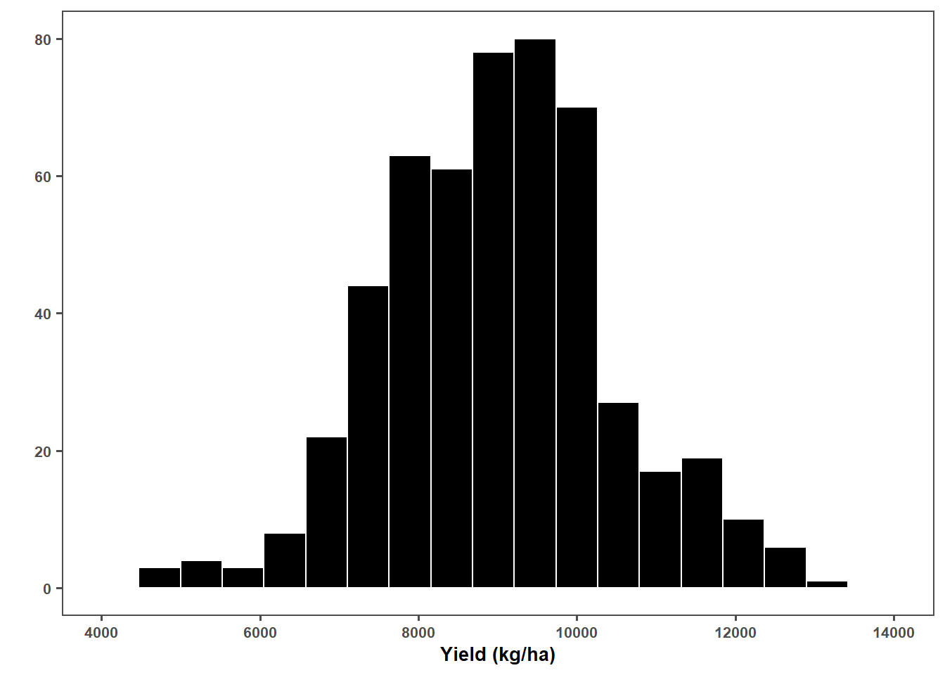

plot_grid(plot_sev, plot_yld, ncol = 2, label_x = -0.03, label_size = 14,
          labels = c("(a)","(b)"))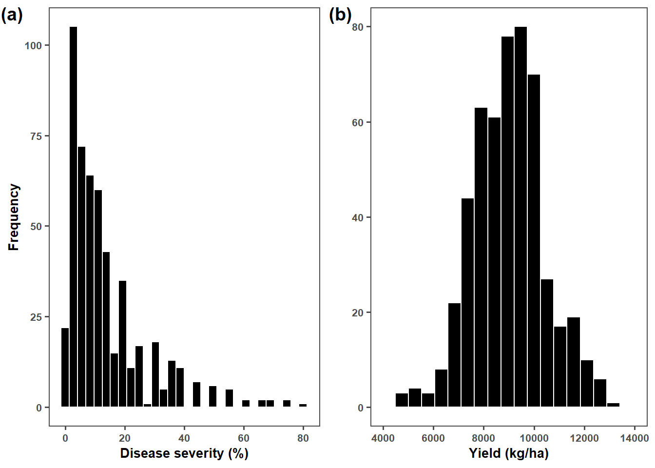

ggsave("fig/sev_yld.png", bg = "white", dpi = 600, 
       width = 8, height = 4)

Prepare data

estria2 <- gls |> 
  group_by(trial, hybrid) |> 
  summarise(mean_sev = mean(sev),
            mean_yld = mean(yld))


max(estria2$mean_sev)

[1] 76.66667

min(estria2$mean_sev)

[1] 1.333333

mean(estria2$mean_sev)

[1] 13.83716

median(estria2$mean_sev)

[1] 9.5

sd(estria2$mean_sev)

[1] 13.12138

max(estria2$mean_yld)

[1] 12503.86

min(estria2$mean_yld)

[1] 3909.777

mean(estria2$mean_yld)

[1] 8964.191

median(estria2$mean_yld)

[1] 8989.737

sd(estria2$mean_yld)

[1] 1359.003

Visualize

estria2 = estria2 %>% 
  mutate(
    period = case_when(trial == "2018_1"~ "2018/1",
                       trial == "2018_2" ~"2018/2",
                       trial == "2018_19"~"2018/2019",
                       trial == "2019_1" ~"2019/1"))
library(ggthemes)

 trials = estria2 |>
  ggplot(aes(mean_sev, mean_yld, group = as.factor(period),color = as.factor(period)))+ #
  geom_point()+
  #facet_wrap(~period)+
  geom_smooth(method = "lm", se = FALSE, size = 2)+
  scale_color_viridis_d()+
  theme_minimal()+
   scale_y_continuous(breaks = c(4000, 5000,6000,7000,8000,9000,10000,11000,12000), 
                     limits = c(4000, 12000))+
  theme_few()+
  labs(x = "Disease severity (%)",
       y = "Yield (kg/ha)",
       color = "Seasons")+
  theme(text = element_text(size = 12, face = "bold"),
        legend.position = "none")
  #geom_abline(slope = -49.3, intercept = 9714, linetype = 1, linewidth =2, color = "gray50")

ggsave("fig/trials.png", bg = "white", dpi = 600, 
       width = 6, height = 4)

library(broom)
lmer_stats = estria2 %>%
  #group_by(year) %>%
  dplyr::select(trial, mean_yld,mean_sev) %>%
  group_by(trial) %>%
  do({
    model <- lm(.$mean_yld ~ .$mean_sev)
    tidy_model <- tidy(model)
    confint_model <- confint(model)  # Calcula os intervalos de confiança
    bind_cols(tidy_model, confint_model)
  })




lmer_stats = lmer_stats |> 
filter(term %in% c("(Intercept)",".$mean_sev"))
 
lmer_stats[lmer_stats$term== "(Intercept)",c("parameters")] <- "Intercept"
lmer_stats[lmer_stats$term== ".$mean_sev",c("parameters")] <- "Slope"

i <- 1
 while (i <= nrow(lmer_stats)) {
  if (lmer_stats$parameters[i] == "Slope" && lmer_stats$estimate[i] > 0) {
    # Remove a linha do Slope e a linha do Intercept correspondente
    lmer_stats <- lmer_stats[-c(i, i - 1), ]
    # Atualiza o índice, pois duas linhas foram removidas
    i <- i - 2
  }
  i <- i + 1
 }
lmer_stats

slope_trial_m= lmer_stats |> 
  filter(parameters == "Slope") %>% 
  summarise(
    Slope = estimate
  )

slope_trial_m[,1] = NULL

slope_trial_m |> 
  filter(!Slope == "NA") |> 
  summarise(
mean = mean(Slope))

intercept_trial_m = lmer_stats |> 
  filter(parameters == "Intercept") %>%  
  summarise(
    Intercept = estimate
  )
intercept_trial_m[,1] = NULL

mean(intercept_trial_m$Intercept)

[1] 9711.667

regression_trial_m = cbind(slope_trial_m,intercept_trial_m)
regression_trial_m[,3] = NULL

summary_stats <- regression_trial_m %>%
  reframe(
    mean_intercept = mean(Intercept),
    mean_slope = mean(Slope),
    ci_intercept_lower = quantile(Intercept, 0.025),
    ci_intercept_upper = quantile(Intercept, 0.975),
    ci_slope_lower = quantile(Slope, 0.025),
    ci_slope_upper = quantile(Slope, 0.975)
  )

trials = estria2|> 
 ggplot(aes(mean_sev, y = mean_yld)) +
  geom_point(color = "NA")+
  scale_y_continuous(breaks = c(4000,6000,8000,10000,12000), 
                     limits = c(4000, 12000))+
  geom_abline(data =regression_trial_m, aes(slope = Slope, intercept = Intercept), size = 1,
              alpha = 0.5, color = "grey")+##9ccb86
  #geom_abline(data =summary_stats, aes(slope = mean_slope, intercept = mean_intercept),
   #           size = 1.5, fill = "black", color = "black")+
geom_abline(data = summary_stats,aes(intercept = ci_intercept_lower,slope = ci_slope_lower) ,
              size = 1.5, linetype = 2, fill = "grey", color = "grey")+
  geom_abline(data = summary_stats, aes(intercept = ci_intercept_upper,slope = ci_slope_upper), size = 1.5, linetype = 2, fill = "grey", color = "grey")+
  geom_abline(aes(slope = -49.37, intercept = 9714.0),
              size = 1.5, fill = "black", color = "black")+
geom_abline(aes(intercept = 8699.1,slope = -60.59) ,
              size = .51, linetype = 2)+
  geom_abline(aes(intercept = 10733.8,slope = -38.00), size = .51, linetype = 2)+
  ggthemes::theme_few()+
  theme(text = element_text(size = 10, face = "bold"),
        axis.title = element_text(size = 10, face = "bold"),
        legend.position = "none")+
  labs(x = "Disease severity (%)", y = "Attainable yield (kg/ha)",
       title = "")

first_plot = estria2 |> 
  filter(trial == "2018_1") %>% 
  ggplot(aes(mean_sev, mean_yld))+ #, group = trial, color = trial
  geom_point()+
  facet_wrap(~trial)+
  geom_smooth(method = "lm", se = FALSE, size = 2, color = "black")+
  scale_x_continuous(breaks = c(0, 20, 40,60,80), limits = c(0, 80))+
  scale_y_continuous(breaks = c(5000, 7500, 10000,12500), limits = c(5000, 12500))+
  scale_color_viridis_d()+
  theme_minimal()+
  theme_few()+
  labs(x = "Severity (%)",
       y = "Yield (kg/ha)",
       color = "Trial")+
  theme(text = element_text(size = 12, face = "bold"))

second_plot = estria2 |> 
  filter(trial == "2018_2") %>% 
  ggplot(aes(mean_sev, mean_yld))+ #, group = trial, color = trial
  geom_point()+
  facet_wrap(~trial)+
  geom_smooth(method = "lm", se = FALSE, size = 2, color = "black")+
  scale_x_continuous(breaks = c(0, 20, 40,60,80), limits = c(0, 80))+
  scale_y_continuous(breaks = c(5000, 7500, 10000,12500), limits = c(5000, 12500))+
  scale_color_viridis_d()+
  theme_minimal()+
  theme_few()+
  labs(x = "Severity (%)",
       y = "Yield (kg/ha)",
       color = "Trial")+
  theme(text = element_text(size = 12, face = "bold"))

third_plot = estria2 |> 
  filter(trial == "2018_19") %>% 
  ggplot(aes(mean_sev, mean_yld))+ #, group = trial, color = trial
  geom_point()+
  facet_wrap(~trial)+
  geom_smooth(method = "lm", se = FALSE, size = 2, color = "black")+
  scale_x_continuous(breaks = c(0, 20, 40,60,80), limits = c(0, 80))+
  scale_y_continuous(breaks = c(5000, 7500, 10000,12500), limits = c(5000, 12500))+
  scale_color_viridis_d()+
  theme_minimal()+
  theme_few()+
  labs(x = "Severity (%)",
       y = "Yield (kg/ha)",
       color = "Trial")+
  theme(text = element_text(size = 12, face = "bold"))

fourth_plot = estria2 |> 
  filter(trial == "2019_1") %>% 
  ggplot(aes(mean_sev, mean_yld))+ #, group = trial, color = trial
  geom_point()+
  facet_wrap(~trial)+
  geom_smooth(method = "lm", se = FALSE, size = 2, color = "black")+
  scale_x_continuous(breaks = c(0, 20, 40,60,80), limits = c(0, 80))+
  scale_y_continuous(breaks = c(5000, 7500, 10000,12500), limits = c(5000, 12500))+
  scale_color_viridis_d()+
  theme_minimal()+
  theme_few()+
  labs(x = "Severity (%)",
       y = "Yield (kg/ha)",
       color = "Trial")+
  theme(text = element_text(size = 12, face = "bold"))

library(patchwork)

combined_plot <- (first_plot | plot_yld | second_plot) / 
                 (third_plot | plot_sev | fourth_plot) +
                 plot_layout(widths = c(2, 10, 2), heights = c(1, 1))
combined_plot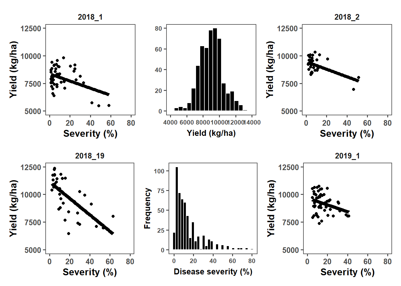

ggsave("fig/plot_all.png", bg = "white", width = 10, height = 8)

Modeling

Fitting

library(lme4)

# Fit a mixed-effects model
obs_model_lmer <- lmer(mean_yld ~ mean_sev + (1 | trial), data = estria2)


# Summary of the model
summary(obs_model_lmer)

Linear mixed model fit by REML ['lmerMod']
Formula: mean_yld ~ mean_sev + (1 | trial)
   Data: estria2

REML criterion at convergence: 2880.3

Scaled residuals: 
    Min      1Q  Median      3Q     Max 
-3.4362 -0.7056  0.0671  0.7105  2.0247 

Random effects:
 Groups   Name        Variance Std.Dev.
 trial    (Intercept) 820678   905.9   
 Residual             941736   970.4   
Number of obs: 174, groups:  trial, 4

Fixed effects:
            Estimate Std. Error t value
(Intercept) 9714.049    465.870  20.851
mean_sev     -49.378      5.745  -8.595

Correlation of Fixed Effects:
         (Intr)
mean_sev -0.168

confint(obs_model_lmer)

                 2.5 %      97.5 %
.sig01       426.84166  1944.19893
.sigma       873.17446  1080.29427
(Intercept) 8699.18638 10733.83869
mean_sev     -60.59337   -38.00271

set.seed(1234)

# Parameters from the fitted model
fixed_intercept <- 9714.049
fixed_slope <- -49.378
random_effect_sd <- 905.9  # sqrt(820678)
residual_sd <- 970.4       # sqrt(941736)

# Number of experiments and points per experiment
num_experiments <- 200  # New experiments
points_per_experiment <- 50

# Simulate data
# Get the range of observed severity values from the original dataset
set.seed(123)

# Simulate data with variable max severity for each experiment
simulated_data_lmer <- data.frame()
for (exp in 1:num_experiments) {
  # Simulate random intercept for the experiment
  u_j <- rnorm(1, mean = 0, sd = random_effect_sd)
  
  # Randomly select a max severity for this simulation between 50% and 80%
  max_sev_sim <- runif(1, min = 20, max = 80)
  
  # Simulate severity values (independent variable) within the 0 to max_sev_sim range
  sev <- runif(points_per_experiment, min = 0, max = max_sev_sim)

  # Simulate residuals
  residuals <- rnorm(points_per_experiment, mean = 0, sd = residual_sd)
  
  # Generate yield (dependent variable)
  yld <- fixed_intercept + u_j + fixed_slope * sev + residuals
  
  # Combine into a data frame
  exp_data <- data.frame(experiment = paste0("Exp_", exp), sev = sev, yld = yld)
  simulated_data_lmer <- rbind(simulated_data_lmer, exp_data)
}

simulated_data_lmer$hybrid <- paste0("hybrid_", sprintf("%02d", (seq_len(nrow(simulated_data_lmer)) - 1) %/% 50 + 1))
# View simulated data
head(simulated_data_lmer)

summary(simulated_data_lmer)

  experiment             sev                yld           hybrid         
 Length:10000       Min.   : 0.00051   Min.   : 2528   Length:10000      
 Class :character   1st Qu.:10.61846   1st Qu.: 7391   Class :character  
 Mode  :character   Median :21.04083   Median : 8509   Mode  :character  
                    Mean   :24.67849   Mean   : 8472                     
                    3rd Qu.:36.17231   3rd Qu.: 9594                     
                    Max.   :78.27768   Max.   :14239                     

library(ggplot2)

# Compare simulated and real severity-yield relationships
ggplot(simulated_data_lmer, aes(x = sev, y = yld, color = experiment)) +
  geom_point(alpha = 0.5) +
  geom_smooth(method = "lm", se = FALSE) +
  theme_minimal() +
  theme(legend.position = "none")+
  labs(title = "Simulated Severity-Yield Data", x = "Severity", y = "Yield")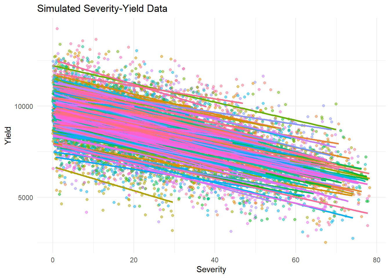

simu_model_lmer <- lmer(yld ~ sev + (1 | experiment), data = simulated_data_lmer)
simu_model_lmer

Linear mixed model fit by REML ['lmerMod']
Formula: yld ~ sev + (1 | experiment)
   Data: simulated_data_lmer
REML criterion at convergence: 166620.8
Random effects:
 Groups     Name        Std.Dev.
 experiment (Intercept) 937.3   
 Residual               966.9   
Number of obs: 10000, groups:  experiment, 200
Fixed Effects:
(Intercept)          sev  
    9691.01       -49.39  

summary(simu_model_lmer)

Linear mixed model fit by REML ['lmerMod']
Formula: yld ~ sev + (1 | experiment)
   Data: simulated_data_lmer

REML criterion at convergence: 166620.8

Scaled residuals: 
    Min      1Q  Median      3Q     Max 
-3.6504 -0.6689  0.0041  0.6771  3.3524 

Random effects:
 Groups     Name        Variance Std.Dev.
 experiment (Intercept) 878546   937.3   
 Residual               934819   966.9   
Number of obs: 10000, groups:  experiment, 200

Fixed effects:
             Estimate Std. Error t value
(Intercept) 9691.0145    68.8438  140.77
sev          -49.3879     0.6449  -76.59

Correlation of Fixed Effects:
    (Intr)
sev -0.231

confint(simu_model_lmer)

                2.5 %    97.5 %
.sig01       848.3483 1036.5979
.sigma       953.4327  980.5062
(Intercept) 9555.8113 9826.1935
sev          -50.6520  -48.1241

obs_fixed_effects_lmer <- fixef(obs_model_lmer)  # From the original model
simu_fixed_effects_lmer <- fixef(simu_model_lmer)  # From the simulated model

print(obs_fixed_effects_lmer)

(Intercept)    mean_sev 
 9714.04857   -49.37773 

print(simu_fixed_effects_lmer)

(Intercept)         sev 
 9691.01451   -49.38785 

obs_random_effects_lmer <- VarCorr(obs_model_lmer)
simu_random_effects_lmer <- VarCorr(simu_model_lmer)

print(obs_random_effects_lmer)

 Groups   Name        Std.Dev.
 trial    (Intercept) 905.91  
 Residual             970.43  

print(simu_random_effects_lmer)

 Groups     Name        Std.Dev.
 experiment (Intercept) 937.31  
 Residual               966.86  

obs_residual_sd_lmer <- attr(VarCorr(obs_model_lmer), "sc")
simu_residual_sd_lmer <- attr(VarCorr(simu_model_lmer), "sc")

print(obs_residual_sd_lmer)

[1] 970.4308

print(simu_residual_sd_lmer)

[1] 966.8604

Plotting

library(broom)
lmer_stats = simulated_data_lmer %>%
  #group_by(year) %>%
  dplyr::select(experiment, yld,sev) %>%
  group_by(experiment) %>%
  do({
    model <- lm(.$yld ~ .$sev)
    tidy_model <- tidy(model)
    confint_model <- confint(model)  # Calcula os intervalos de confiança
    bind_cols(tidy_model, confint_model)
  })




lmer_stats = lmer_stats |> 
filter(term %in% c("(Intercept)",".$sev"))
 
lmer_stats[lmer_stats$term== "(Intercept)",c("parameters")] <- "Intercept"
lmer_stats[lmer_stats$term== ".$sev",c("parameters")] <- "Slope"

i <- 1
 while (i <= nrow(lmer_stats)) {
  if (lmer_stats$parameters[i] == "Slope" && lmer_stats$estimate[i] > 0) {
    # Remove a linha do Slope e a linha do Intercept correspondente
    lmer_stats <- lmer_stats[-c(i, i - 1), ]
    # Atualiza o índice, pois duas linhas foram removidas
    i <- i - 2
  }
  i <- i + 1
 }
lmer_stats

slope_trial_m= lmer_stats |> 
  filter(parameters == "Slope") %>% 
  summarise(
    Slope = estimate
  )

slope_trial_m[,1] = NULL

slope_trial_m |> 
  filter(!Slope == "NA") |> 
  summarise(
mean = mean(Slope))

intercept_trial_m = lmer_stats |> 
  filter(parameters == "Intercept") %>%  
  summarise(
    Intercept = estimate
  )
intercept_trial_m[,1] = NULL

mean(intercept_trial_m$Intercept)

[1] 9692.539

regression_trial_m = cbind(slope_trial_m,intercept_trial_m)
regression_trial_m[,3] = NULL

summary_stats <- regression_trial_m %>%
  reframe(
    mean_intercept = mean(Intercept),
    mean_slope = mean(Slope),
    ci_intercept_lower = quantile(Intercept, 0.025),
    ci_intercept_upper = quantile(Intercept, 0.975),
    ci_slope_lower = quantile(Slope, 0.025),
    ci_slope_upper = quantile(Slope, 0.975)
  )

lmer_plot = simulated_data_lmer|> 
 ggplot(aes(sev, y = yld)) +
  geom_point(color = "NA")+
  scale_y_continuous(breaks = c(4000,6000,8000,10000,12000), 
                     limits = c(4000, 12000))+
  geom_abline(data =regression_trial_m, aes(slope = Slope, intercept = Intercept), size = 1,
              alpha = 0.5, color = "grey")+##9ccb86
#  geom_abline(data =summary_stats, aes(slope = mean_slope, intercept = mean_intercept),
 #             size = 1.5, fill = "black", color = "black")+
  geom_abline(data = summary_stats,aes(intercept = ci_intercept_lower,slope = ci_slope_lower) ,
              size = 1.5, linetype = 2, fill = "grey", color = "grey")+
  geom_abline(data = summary_stats, aes(intercept = ci_intercept_upper,slope = ci_slope_upper), size = 1.5, linetype = 2, fill = "grey", color = "grey")+
  geom_abline( aes(slope = -49.38, intercept = 9691.0),
              size = 1.5, fill = "black", color = "black")+
  geom_abline(aes(intercept = 9555.81,slope = -50.65) ,
              size = .51, linetype = 2)+
  geom_abline(aes(intercept = 9826.19,slope = -48.12), size = .51, linetype = 2)+
   ggthemes::theme_few()+
  theme(text = element_text(size = 10, face = "bold"),
        axis.title = element_text(size = 10, face = "bold"),
        legend.position = "none")+
  labs(x = "Disease severity (%)", y = "",
       title = "")

lmer_plot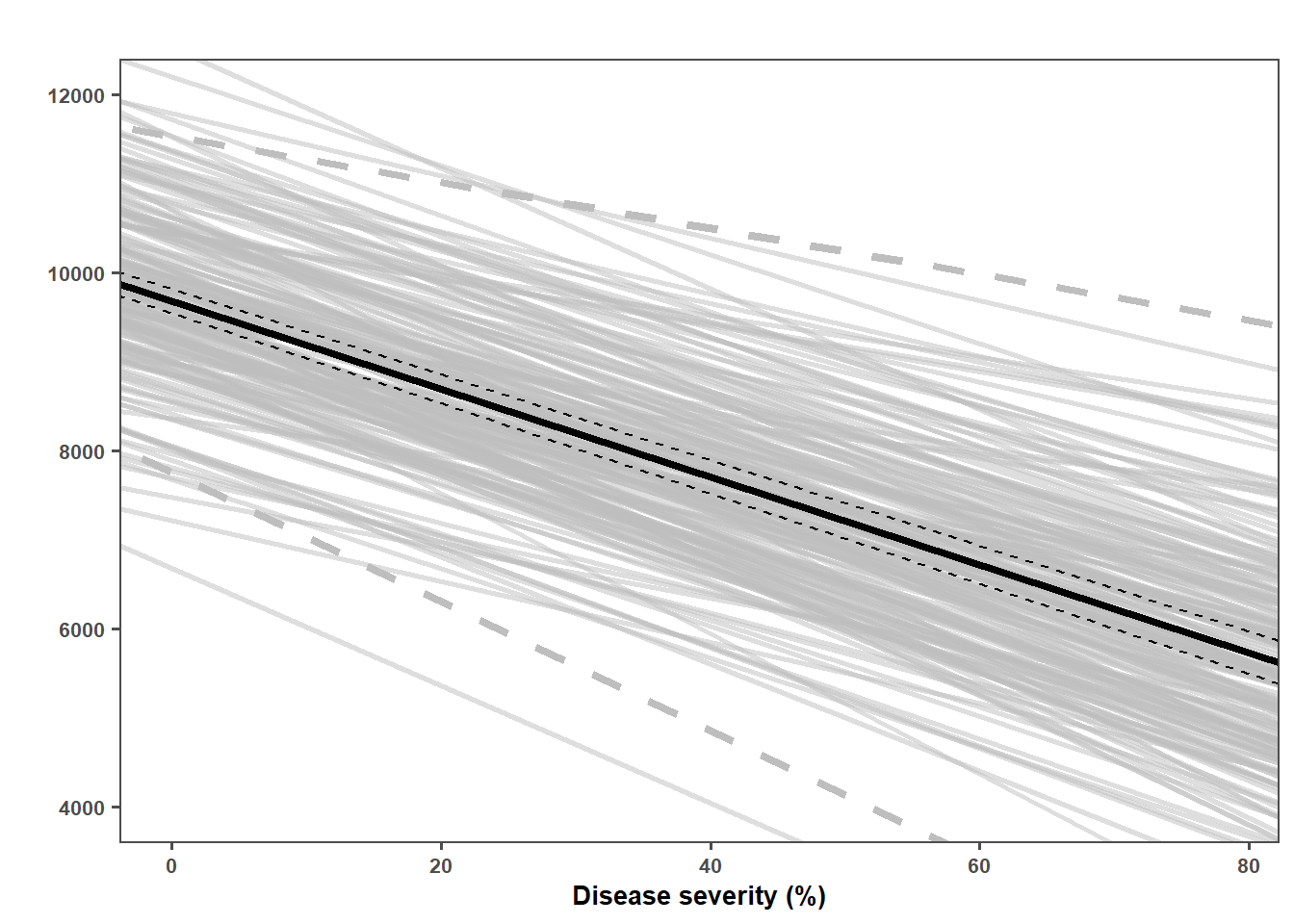

Joining

plot_grid(trials,lmer_plot,plot_sev, plot_yld, labels = c("(a)","(b)","(c)","(d)"), ncol = 2,
          label_size = 10, label_x = -0.01)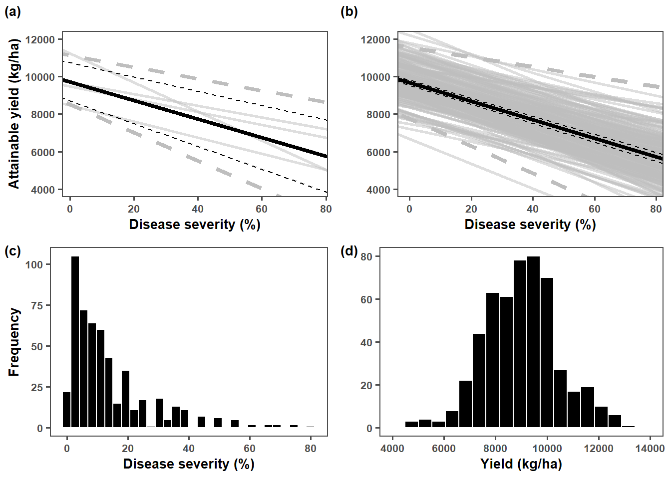

ggsave("fig/obs_simu_model.png", bg = "white", dpi = 600,width = 6, height = 4)

cor(estria2$mean_sev, estria2$mean_yld)

[1] -0.4051456

cor(simulated_data_lmer$sev, simulated_data_lmer$yld)

[1] -0.5508678

Performance

Empirical

obs_lmer_predicted <- predict(obs_model_lmer)


obs_lmer_observed <- estria2$mean_yld


obs_lmer_residuals <- obs_lmer_observed - obs_lmer_predicted


obs_lmer_RMSE <- sqrt(mean(obs_lmer_residuals^2))  
obs_lmer_MAE <- mean(abs(obs_lmer_residuals))     
obs_lmer_correlation <- cor(obs_lmer_observed, obs_lmer_predicted)

performance::check_normality(obs_model_lmer)

OK: residuals appear as normally distributed (p = 0.227).

performance::check_heteroscedasticity(obs_model_lmer)

Warning: Heteroscedasticity (non-constant error variance) detected (p < .001).

performance::check_autocorrelation(obs_model_lmer)

Warning: Autocorrelated residuals detected (p = 0.004).

Simulated

simu_lmer_predicted <- predict(simu_model_lmer)


simu_lmer_observed <- simulated_data_lmer$yld


simu_lmer_residuals <- simu_lmer_observed - simu_lmer_predicted


simu_lmer_RMSE <- sqrt(mean(simu_lmer_residuals^2))  
simu_lmer_MAE <- mean(abs(simu_lmer_residuals))     
simu_lmer_correlation <- cor(simu_lmer_observed, simu_lmer_predicted)       

performance::check_normality(simu_model_lmer)

OK: residuals appear as normally distributed (p = 0.875).

performance::check_heteroscedasticity(simu_model_lmer)

Warning: Heteroscedasticity (non-constant error variance) detected (p < .001).

performance::check_autocorrelation(simu_model_lmer)

Warning: Autocorrelated residuals detected (p < .001).

Visualization

Simulated

# Extrair os resíduos e quantis teóricos
lmer_residuals <- residuals(simu_model_lmer, type = "deviance")
lmer_qq_data <- data.frame(
  theoretical = qqnorm(lmer_residuals, plot.it = FALSE)$x*1000,
  residuals = qqnorm(lmer_residuals, plot.it = FALSE)$y
)

# Plotar o QQ plot
lmer_qq = lmer_qq_data %>% 
  ggplot(aes(x = theoretical, y = residuals)) +
  geom_point() +
  geom_abline(intercept = 0, slope = 1, color = "red", linetype = "dashed") +
  scale_x_continuous(breaks = c(-3000,-2000,-1000,0,1000,2000,3000), 
                     limits = c(-3000, 3000))+
  scale_y_continuous(breaks = c(-3000,-2000,-1000,0,1000,2000,3000), 
                     limits = c(-3000, 3000))+
  labs(x = "Theoretical Quantiles", y = "") +
  ggthemes::theme_few()+
  theme(text = element_text(size = 12, face = "bold"))

lmer_qq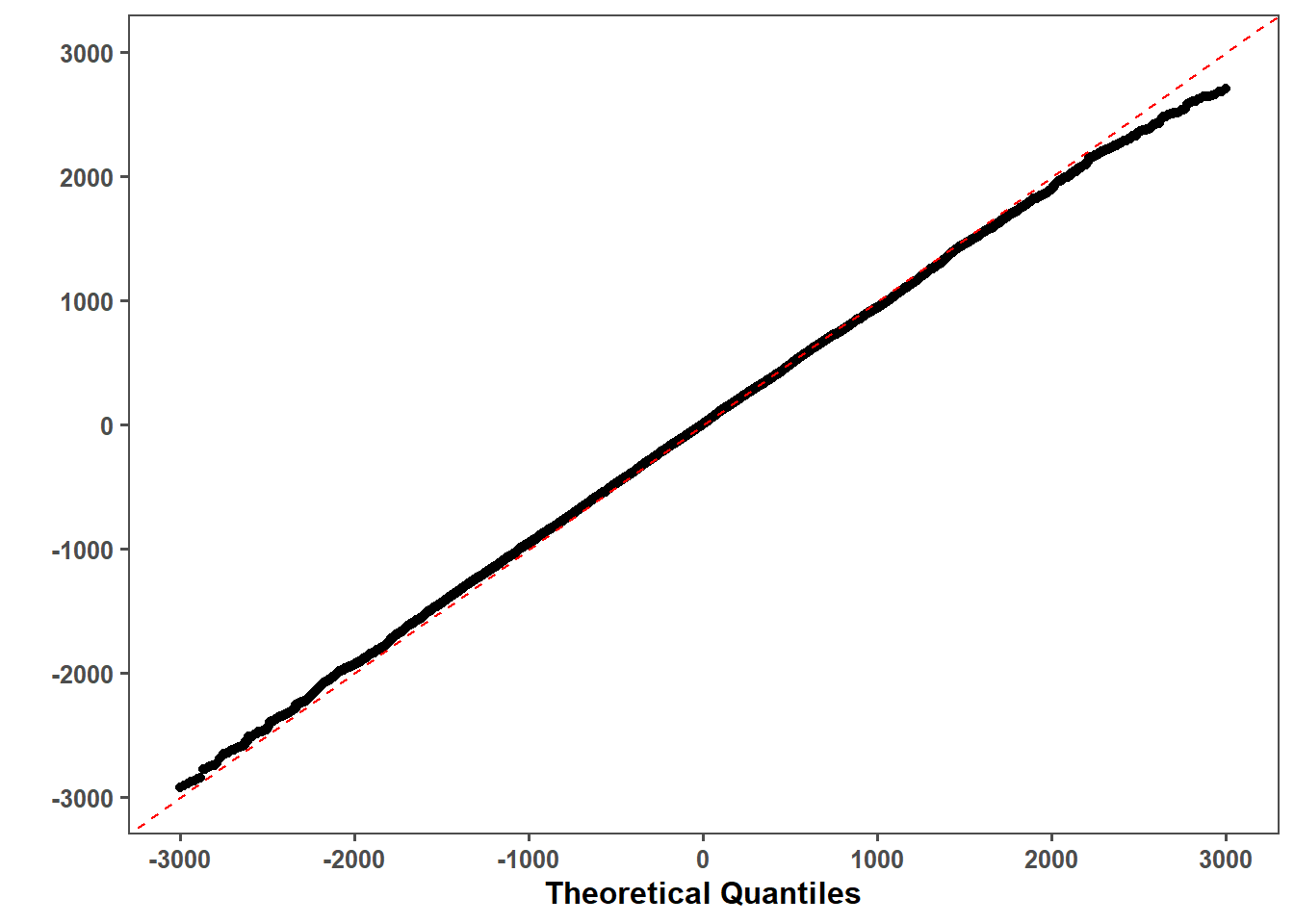

# Extrair preditores lineares e resíduos
lmer_linear_predictors <- predict(simu_model_lmer, type = "link")
lmer_residuals_data <- data.frame(
  linear_predictors = lmer_linear_predictors,
  residuals = lmer_residuals
)

# Plotar resíduos vs preditores lineares
lmer_predictors = lmer_residuals_data %>% 
  ggplot(aes(x = linear_predictors, y = residuals)) +
  geom_point(alpha = 0.2, color = "grey", size = 2) +
  geom_hline(yintercept = 0, color = "black", linetype = "dashed", size = 1.4) +
  scale_x_continuous(breaks = c(4000,6000,8000,10000,12000), 
                     limits = c(4000, 12000))+
  scale_y_continuous(breaks = c(-3000,-2000,-1000,0,1000,2000,3000), 
                     limits = c(-3000, 3000))+
  labs(x = "Linear Predictors", y = "") +
  ggthemes::theme_few()+
  theme(text = element_text(size = 12, face = "bold"))

# Calcular média e desvio-padrão dos resíduos
mean_res <- mean(lmer_residuals_data$residuals)
sd_res <- sd(lmer_residuals_data$residuals)

# Plotar o histograma e a curva acumulada normal
lmer_res_hist <- ggplot(lmer_residuals_data, aes(x = residuals)) +
  geom_histogram(aes(y = ..density..), fill = "black", color = "white", bins = 20) + # Ajusta para densidade
  stat_function(fun = dnorm, args = list(mean = mean_res, sd = sd_res), 
                color = "darkred", size = 1.2, linetype = "solid") + # Adiciona a curva normal
  scale_x_continuous(breaks = c(-2500, -1250, 0, 1250, 2500), 
                     limits = c(-2500, 2500)) +
  labs(x = "Deviance Residuals", y = "") +
  ggthemes::theme_few() +
  theme(text = element_text(size = 12, face = "bold"))

# Exibir o gráfico
lmer_res_hist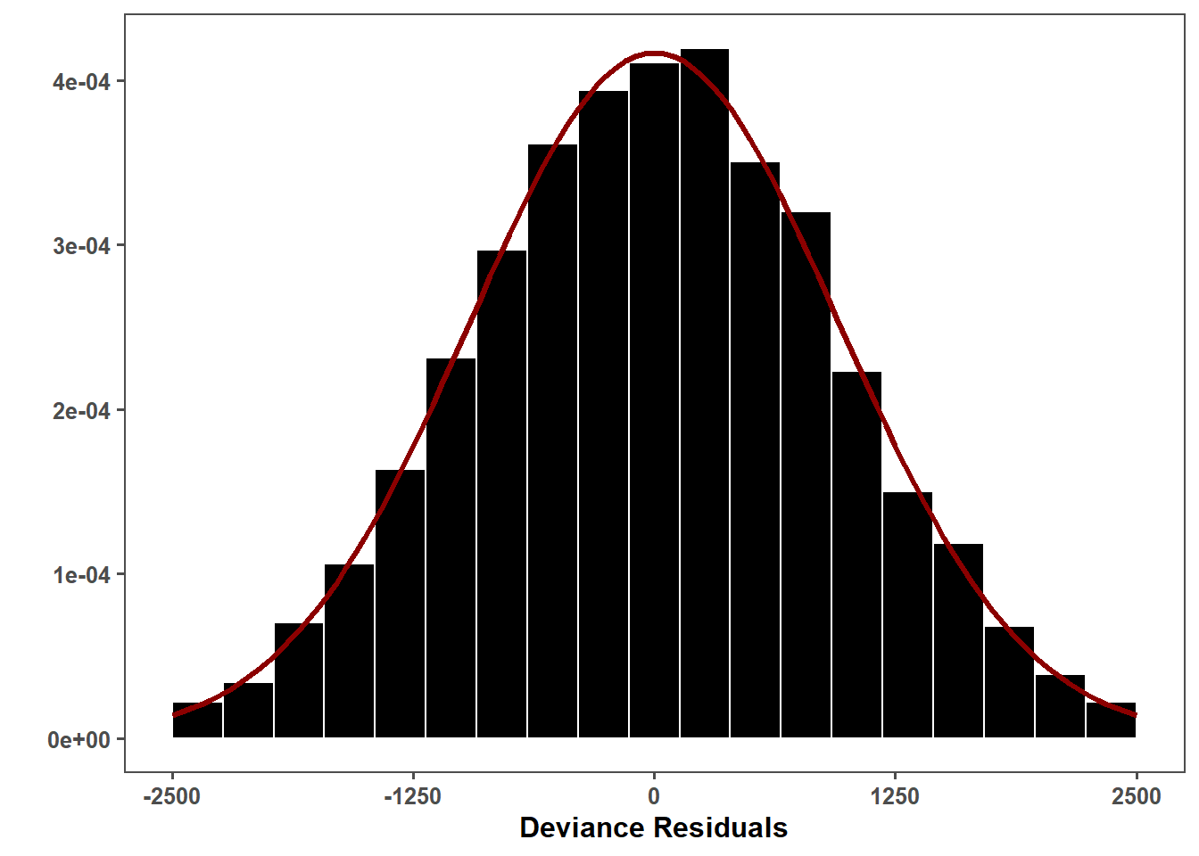

# Extrair valores observados e preditos
lmer_observed <- simulated_data_lmer$yld
lmer_predicted <- predict(simu_model_lmer, type = "response")
lmer_prediction_data <- data.frame(
  observed = lmer_observed,
  predicted = lmer_predicted
)

# Plotar valores preditos vs observados
lmer_pd_ob = lmer_prediction_data %>% 
  ggplot(aes(x = observed, y = predicted)) +
  geom_point(alpha = 0.5, color = "grey", size = 2) +
  geom_abline(intercept = 0, slope = 1, color = "black", linetype = "dashed", size = 1.4) +
  scale_x_continuous(breaks = c(4000,6000,8000,10000,12000), 
                     limits = c(4000, 12000))+
  scale_y_continuous(breaks = c(4000,6000,8000,10000,12000), 
                     limits = c(4000, 12000))+
  labs(x = "Observed", y = "") +
  ggthemes::theme_few()+
  theme(text = element_text(size = 12, face = "bold"))

lmer_pd_ob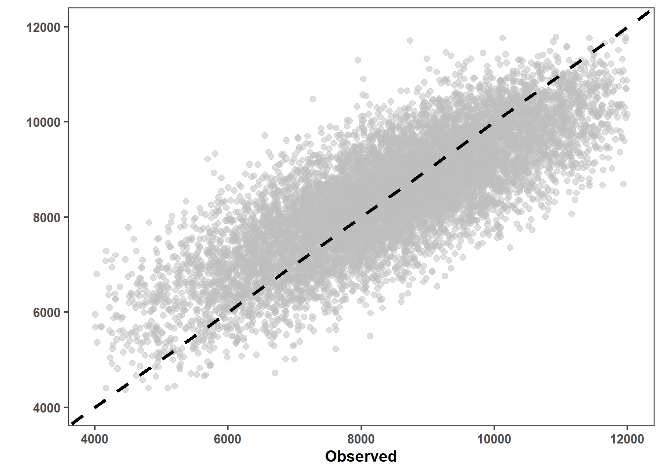

max(lmer_prediction_data$predicted)

[1] 12122.53

Observed

# Extrair os resíduos e quantis teóricos
obs_lmer_residuals <- residuals(obs_model_lmer, type = "deviance")
obs_lmer_qq_data <- data.frame(
  theoretical = qqnorm(obs_lmer_residuals, plot.it = FALSE)$x*1000,
  residuals = qqnorm(obs_lmer_residuals, plot.it = FALSE)$y
)

# Plotar o QQ plot
obs_lmer_qq = obs_lmer_qq_data %>% 
  filter(!residuals < -2000) %>% 
  ggplot(aes(x = theoretical, y = residuals)) +
  geom_point() +
  geom_abline(intercept = 0, slope = 1, color = "red", linetype = "dashed") +
   scale_x_continuous(breaks = c(-3000,-2000,-1000,0,1000,2000,3000), 
                     limits = c(-3000, 3000))+
  scale_y_continuous(breaks = c(-3000,-2000,-1000,0,1000,2000,3000), 
                     limits = c(-3000, 3000))+
  labs(x = "Theoretical Quantiles", y = "Dev. Residuals") +
  ggthemes::theme_few()+
  theme(text = element_text(size = 12, face = "bold"))

obs_lmer_qq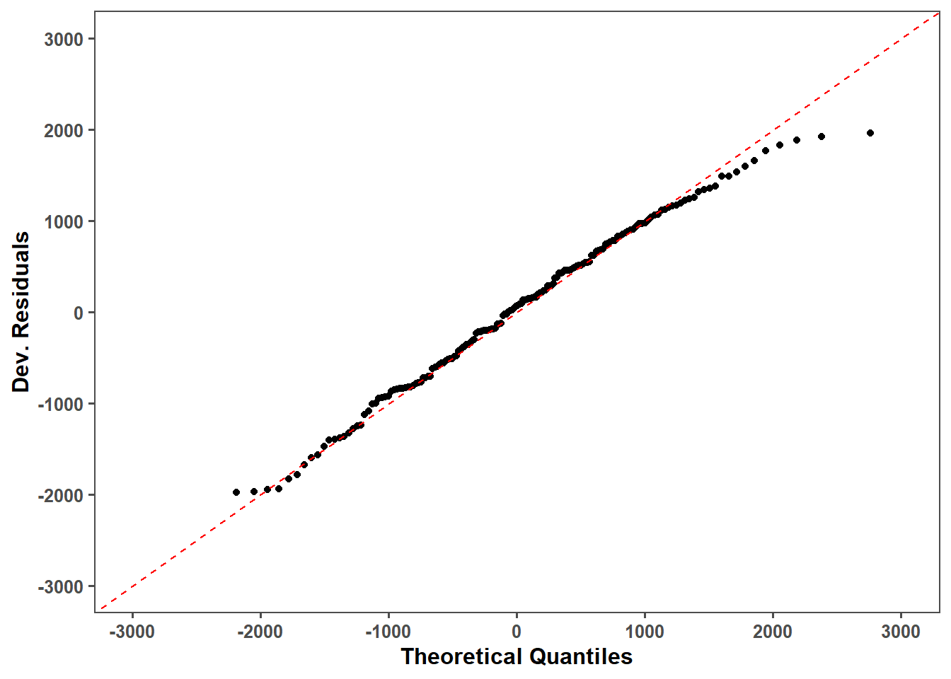

# Extrair preditores lineares e resíduos
obs_lmer_linear_predictors <- predict(obs_model_lmer, type = "link")
obs_lmer_residuals_data <- data.frame(
  linear_predictors = obs_lmer_linear_predictors,
  residuals = obs_lmer_residuals
)

# Plotar resíduos vs preditores lineares
obs_lmer_predictors = obs_lmer_residuals_data %>%
  filter(!residuals < -2000) %>% 
  ggplot(aes(x = linear_predictors, y = residuals)) +
  geom_point(alpha = 0.2, color = "grey", size = 2) +
  geom_hline(yintercept = 0, color = "black", linetype = "dashed", size = 1.4) +
  scale_x_continuous(breaks = c(4000,6000,8000,10000,12000), 
                     limits = c(4000, 12000))+
  scale_y_continuous(breaks = c(-3000,-2000,-1000,0,1000,2000,3000), 
                     limits = c(-3000, 3000))+
  labs(x = "Linear Predictors", y = "Dev. Residuals") +
  ggthemes::theme_few()+
  theme(text = element_text(size = 12, face = "bold"))

# Calcular média e desvio-padrão dos resíduos
mean_res <- mean(obs_lmer_residuals_data$residuals)
sd_res <- sd(obs_lmer_residuals_data$residuals)

# Plotar o histograma e a curva acumulada normal
obs_lmer_res_hist <- ggplot(obs_lmer_residuals_data, aes(x = residuals)) +
  geom_histogram(aes(y = ..density..), fill = "black", color = "white", bins = 20) + # Ajusta para densidade
  stat_function(fun = dnorm, args = list(mean = mean_res, sd = sd_res), 
                color = "darkred", size = 1.2, linetype = "solid") + # Adiciona a curva normal
  scale_x_continuous(breaks = c(-2500, -1250, 0, 1250, 2500), 
                     limits = c(-2500, 2500)) +
  labs(x = "Deviance Residuals", y = "Frequency") +
  ggthemes::theme_few() +
  theme(text = element_text(size = 12, face = "bold"))

# Exibir o gráfico
obs_lmer_res_hist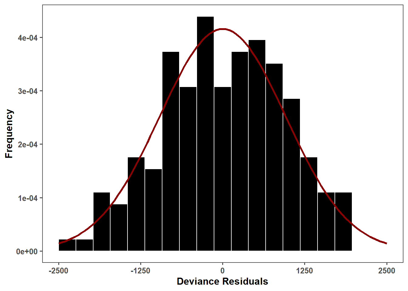

# Extrair valores observados e preditos
obs_lmer_observed <- estria2$mean_yld
obs_lmer_predicted <- predict(obs_model_lmer, type = "response")
obs_lmer_prediction_data <- data.frame(
  observed = obs_lmer_observed,
  predicted = obs_lmer_predicted
)

# Plotar valores preditos vs observados
obs_lmer_pd_ob = obs_lmer_prediction_data %>% 
  ggplot(aes(x = observed, y = predicted)) +
  geom_point(alpha = 0.5, color = "grey", size = 2) +
  geom_abline(intercept = 0, slope = 1, color = "black", linetype = "dashed", size = 1.4) +
  scale_x_continuous(breaks = c(4000,6000,8000,10000,12000), 
                     limits = c(4000, 12000))+
  scale_y_continuous(breaks = c(4000,6000,8000,10000,12000), 
                     limits = c(4000, 12000))+
  labs(x = "Observed", y = "Predicted") +
  ggthemes::theme_few()+
  theme(text = element_text(size = 12, face = "bold"))

obs_lmer_pd_ob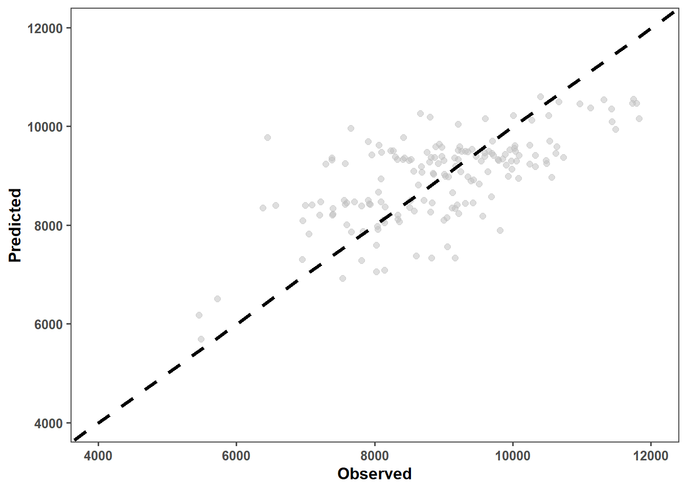

Plotting

#plot_grid(obs_lmer_pd_ob,lmer_pd_ob,
 #         obs_lmer_qq,lmer_qq,
  #        obs_lmer_predictors,lmer_predictors,
   #       obs_lmer_res_hist,lmer_res_hist, ncol = 2, labels = c("a"),
    #      label_x = -0.01,label_y = 0.01)

(obs_lmer_pd_ob | lmer_pd_ob) / 
(obs_lmer_qq | lmer_qq) / 
(obs_lmer_predictors | lmer_predictors) / 
(obs_lmer_res_hist | lmer_res_hist) +
  plot_annotation(tag_levels = "a", tag_prefix = "(", tag_suffix = ")") &
  theme(plot.tag = element_text(face = "bold", size = 14))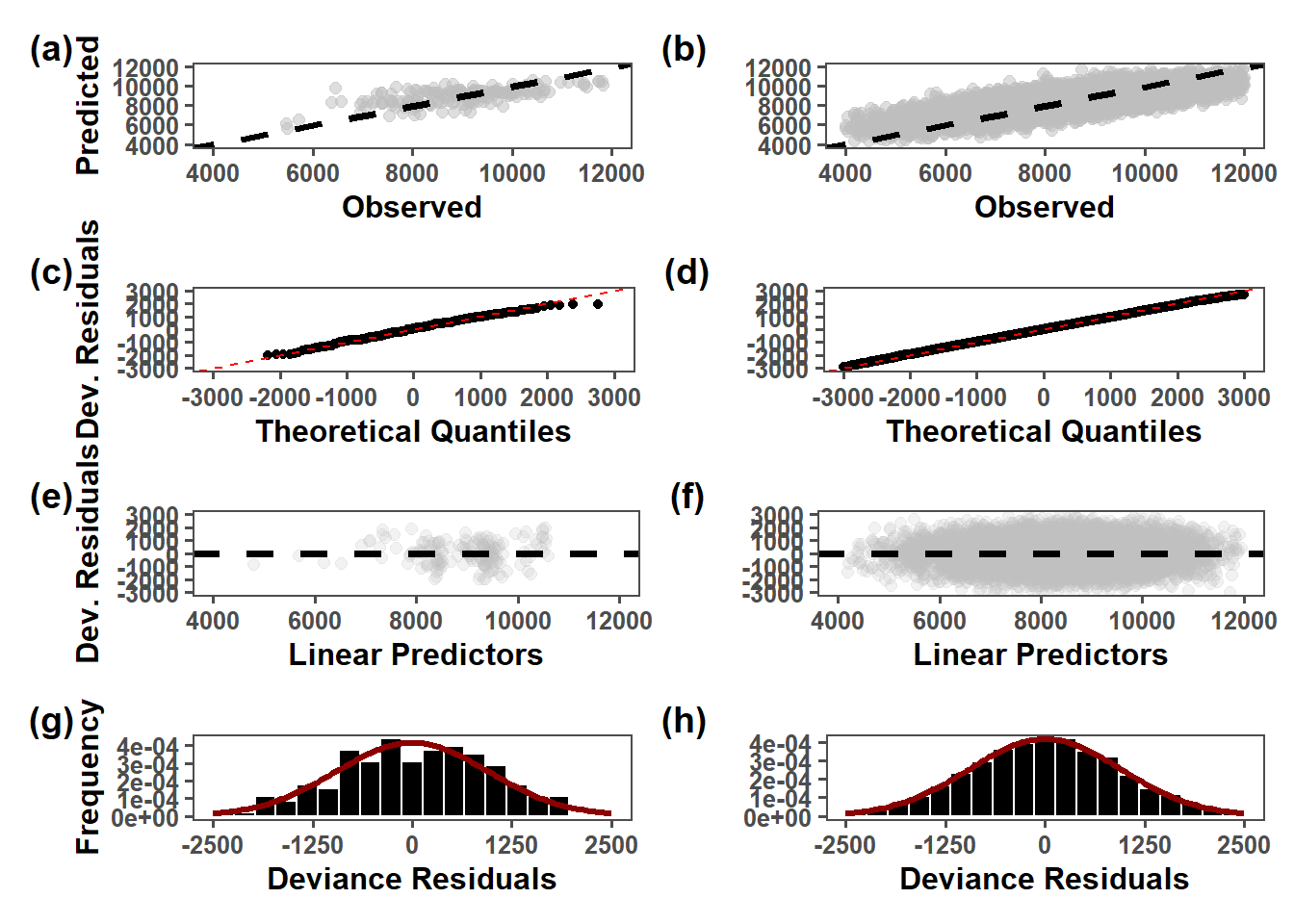

ggsave("fig/lmm_residue.png", dpi = 600, bg = "white", height = 6, width = 8)

Power analysis of model by simulation

Severity

library(simr)
library(ggplot2)
library(dplyr)

# Ajuste do modelo original
sev_lmer <- lmer(mean_yld ~ mean_sev + (1 | trial), data = estria2)

# Criar um modelo extendido para simulação
ext_sev_lmer <- extend(sev_lmer, along = "mean_sev", n = 10000)

# Rodar várias simulações do powerCurve e armazenar os resultados
num_simulations <- 50  # Número de simulações individuais
power_results <- list()

for (i in 1:num_simulations) {
  power_results[[i]] <- as.data.frame(summary(powerCurve(ext_sev_lmer, 
                                                          along = "mean_sev", 
                                                          nsim = 100, 
                                                          breaks = 1:100)))
}


power_df <- bind_rows(power_results, .id = "simulation")

#write_xlsx(power_df, "data/power_df.xlsx")

power_df = read_xlsx("data/power_df.xlsx")


power_df2 <- power_df %>%
  group_by(nlevels) %>%
  summarise(mean = mean(mean, na.rm = TRUE),
            lower = mean(lower, na.rm = TRUE),
            upper = mean(upper, na.rm = TRUE))

power_df %>% 
  filter(mean >= 0.80 & mean <=0.85)

Plotting

ggplot() +
  # Linhas cinzas para cada simulação individual
  geom_line(data = power_df, aes(x = nlevels, y = mean * 100, group = simulation), 
            color = "gray", alpha = 0.4) +
  # Linha da média (laranja)
  geom_line(data = power_df2, aes(x = nlevels, y = mean * 100), 
            color = "black", size = 1.2) +
  # Linhas superior e inferior (preto, tracejado)
  geom_line(data = power_df2, aes(x = nlevels, y = upper * 100), 
            color = "black", linetype = "dashed", size = 0.8) +
  geom_line(data = power_df2, aes(x = nlevels, y = lower * 100), 
            color = "black", linetype = "dashed", size = 0.8)+
  scale_x_continuous(breaks = c(0,5,10,15,20,25,30,35,40,45,50), limits = c(0, 50))+
  scale_y_continuous(breaks = c(0,10,20,30,40,50,
                                60,70,80,90,100), limits = c(0, 100))+
  geom_hline(yintercept = 80, linetype = "dashed", size = 1, color = "darkblue")+
  geom_vline(xintercept = c(25), linetype = 2, size = 1, color = "darkblue")+
  coord_cartesian(xlim = c(0,50))+
  ggthemes::theme_few()+
  theme(text = element_text(size = 12, face = "bold"),
        legend.position = "none")+
  labs(x = "Disease severity (%)",
       y = "Power (%)")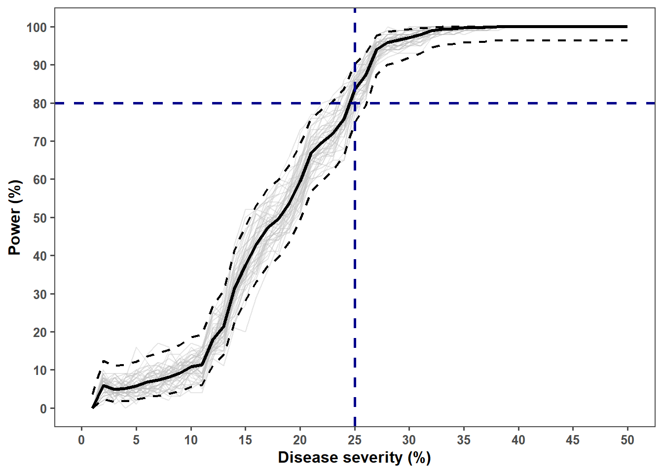

ggsave("fig/power_model.png", bg = "white", dpi = 600,width = 6, height = 4)

Damage

Economic losses

sev  = data.frame(sev = seq(20,100, by = 10))
yield = data.frame(yld = seq(4000,12000,by = 500))
price = data.frame(price = seq(100,300, by = 100))

combined_data <- expand.grid(sev = sev$sev, yld = yield$yld, price = price$price)

ylmer_simu_min = combined_data %>% 
  mutate(loss =((((((49.3/9691.0)*sev)*100)*yld)/100)/1000)*price)


custom_labels <- c(
  "100" = "100 USD/ton",
  "200" = "200 USD/ton",
  "300" = "300 USD/ton"
)


 heat_loss =ylmer_simu_min %>%
   filter(price == "200") %>% 
  ggplot(aes(sev,yld, fill = loss)) +
  geom_tile(color = "white", size = 0.8) +
  scale_x_continuous(breaks = seq(20, 100, by = 10)) +
  scale_y_continuous(breaks = seq(4000, 12000, by = 500)) +
  scale_fill_viridis_b(option = "E", 
                     guide = guide_colorbar(barwidth = 0.3, barheight = 15), 
                     breaks = seq(0, 2000, by = 300))+
   geom_text(aes(label = as.integer(loss)),
    size = 3, colour = "white")+
   #facet_wrap(~price, labeller = as_labeller(custom_labels))+
  theme_minimal_grid(font_size = 14) +
  labs(
    y = "Attainable yield (kg/ha)",
    x = "Disease severity (%)",
    fill = "L (USD/ha)"
  )+
   theme(text = element_text(size = 14),
     axis.title = element_text(size = 20, face = "bold"),
    strip.text = element_text(size= 14, vjust = -1),
    #axis.text.y = element_text(hjust = -3),
    axis.text.x = element_text(vjust = 3),
    legend.position = "right",
    legend.justification = 0.5,
    panel.grid = element_blank())

hist_loss = ylmer_simu_min |>
  filter(price == "200") %>% 
  ggplot(aes(loss))+
  geom_histogram(color = "white", fill= "#1c1c3c", bins = 15)+
  facet_wrap(~price)+
  ggthemes::theme_few() +
   scale_x_continuous(breaks = seq(0,2100, by = 300)) +
  labs(
    y = "Frequency",
    x = "Economic losses (USD/ha)")+
    theme(
    text = element_text(face = "bold", size = 14),
    axis.title = element_text(size = 20, face = "bold"),
    axis.text.x = element_text(vjust = 1, size = 14, face = "bold"),
    axis.text.y = element_text(vjust = 1, size = 14, face = "bold"),
    legend.position = "none",
    legend.justification = 0.5,
    panel.grid = element_blank(),
    strip.text = element_blank() 
  )

loss_200 = ylmer_simu_min |>
  filter(price == "200") 

median(loss_200$loss)

[1] 447.6731

hist_loss = ylmer_simu_min %>% 
  filter(price == "200") %>%
ggplot(aes(x = loss)) +
  stat_halfeye(fill = "#ffc425", alpha = 0.7)+
  geom_vline(aes(xintercept = 447.6731), color = "#1c1c3c", linetype = "dashed", size = 2) +
  ggthemes::theme_few() +
   #scale_x_continuous(breaks = seq(0,2100, by = 100)) +
  scale_x_continuous(breaks=c(50,150,250,350,450,550,
                              650,750,850,950,1050,
                              1150,1250,1350,1450,1550,1650,1750,1850,1950,
                              2150))+
  labs(
    y = "Density",
    x = "Economic losses (USD/ha)")+
    theme(
    text = element_text(face = "bold", size = 14),
    axis.title = element_text(size = 20, face = "bold"),
    axis.text.x = element_text(vjust = 1, size = 14, face = "bold"),
    axis.text.y = element_text(vjust = 1, size = 14, face = "bold"),
    legend.position = "none",
    legend.justification = 0.5,
    panel.grid = element_blank(),
    strip.text = element_blank() 
  )

# Below 25%

sev_loss_b25  = data.frame(sev = seq(5,25, by = 5))

combined_data_b25 <- expand.grid(sev = sev_loss_b25$sev, yld = yield$yld)

loss_25 = ((((((49.3/9691.0)*25)*combined_data_b25$sev)*combined_data_b25$yld)/100)/1000)*200

mean(loss_25)

[1] 30.52317

min(loss_25)

[1] 5.087194

max(loss_25)

[1] 76.30791

# Above 25%

sev_loss_a25  = data.frame(sev = seq(25,100, by = 5))

combined_data_a25 <- expand.grid(sev = sev_loss_a25$sev, yld = yield$yld)

loss_25 = ((((((49.3/9691.0)*combined_data_a25$sev)*combined_data_a25$sev)*combined_data_a25$yld)/100)/1000)*200

mean(loss_25)

[1] 361.1908

min(loss_25)

[1] 25.43597

max(loss_25)

[1] 1220.927

(hist_loss+heat_loss) +
  plot_annotation(tag_levels = "a", tag_prefix = "(", tag_suffix = ")")&
  theme(plot.tag = element_text(face = "bold", size = 24))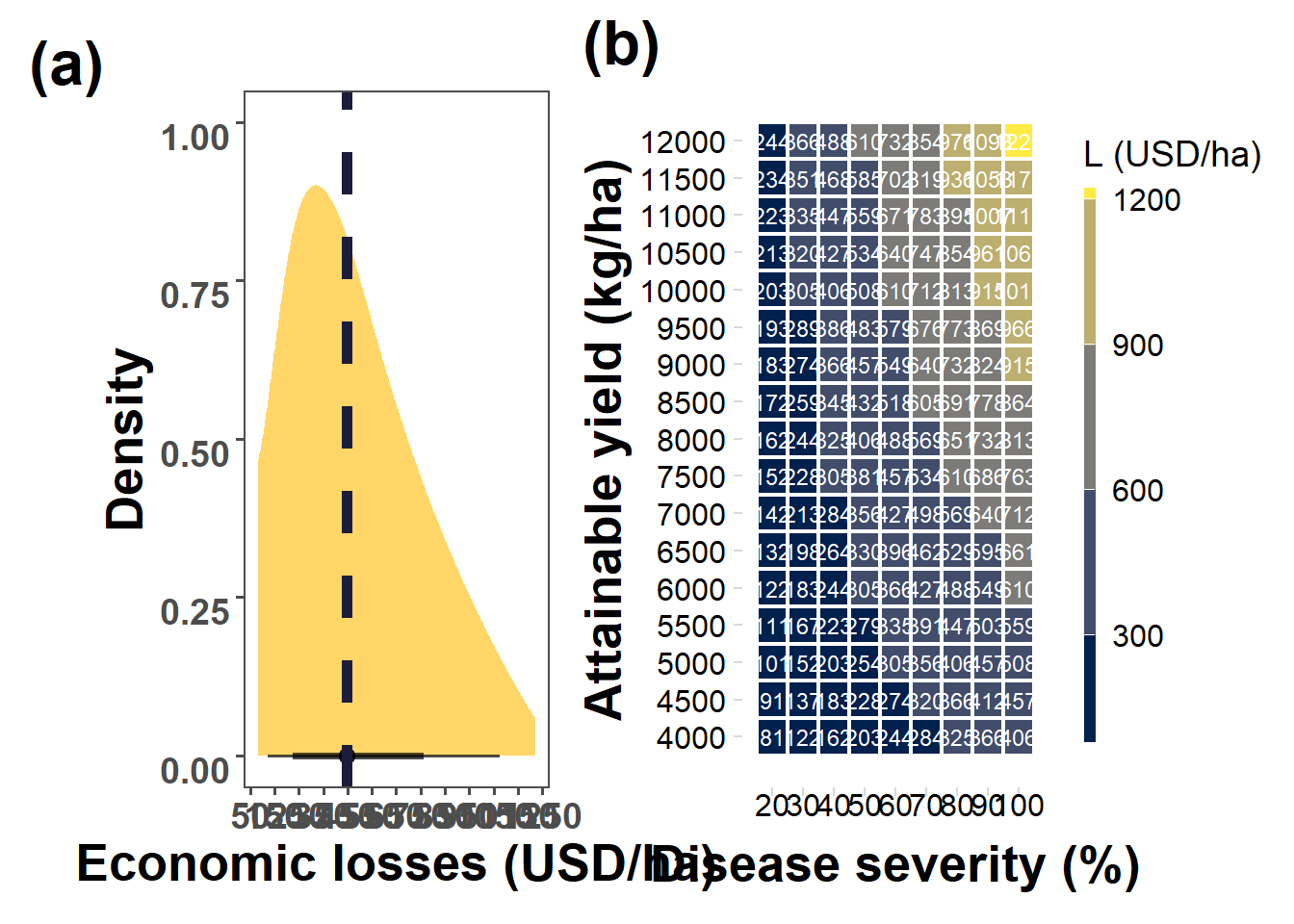 

 ggsave("fig/loss.png", bg = "white",
       dpi = 600,height =8, width = 16)

Relative yield

lmer_slope= lmer_stats %>% 
  filter(parameters == "Slope")

library(minpack.lm)
Fx =environment(ecdf(-lmer_slope$estimate))$y
x = environment(ecdf(-lmer_slope$estimate))$x

slope_reg = nlsLM(Fx ~ pgamma(x, shape, rate,log = FALSE) ,
      start = c(shape = 2.5, rate = 0.13),
      control = nls.lm.control(maxiter = 1024))
summary(slope_reg)

Formula: Fx ~ pgamma(x, shape, rate, log = FALSE)

Parameters:
      Estimate Std. Error t value Pr(>|t|)    
shape 29.25149    0.62746   46.62   <2e-16 ***
rate   0.58169    0.01255   46.37   <2e-16 ***
---
Signif. codes:  0 '***' 0.001 '**' 0.01 '*' 0.05 '.' 0.1 ' ' 1

Residual standard error: 0.02492 on 198 degrees of freedom

Number of iterations to convergence: 12 
Achieved convergence tolerance: 1.49e-08

shape_res = summary(slope_reg)$coef[1]
rate_res = summary(slope_reg)$coef[2]
ks.test(Fx, pgamma(x, shape_res, rate_res))

    Asymptotic two-sample Kolmogorov-Smirnov test

data:  Fx and pgamma(x, shape_res, rate_res)
D = 0.08, p-value = 0.5441
alternative hypothesis: two-sided

slope_plot = lmer_slope %>% 
  ggplot(aes(x = estimate)) +
  geom_histogram(aes(y = ..density..), fill = "black", color = "white", bins = 20) + # Ajusta para densidade
  stat_function(fun=function(x) dgamma(-x, shape_res, rate_res), size = 1.2, color = "darkblue")+
  ggthemes::theme_few()+
  #facet_wrap(~approach)+
  labs(x = "Slope (kg/p.p)",
       y = "Frequency")+
  theme(text = element_text(size = 10, face = "bold"))




lmer_intercept= lmer_stats %>% 
  filter(parameters == "Intercept")

shapiro.test(lmer_slope$estimate)

    Shapiro-Wilk normality test

data:  lmer_slope$estimate
W = 0.98551, p-value = 0.03812

mean_intercept = mean(lmer_intercept$estimate)
sd_intercept = sd(lmer_intercept$estimate)

intercept_plot <- lmer_intercept %>% 
  ggplot(aes(x = estimate)) +
  geom_histogram(aes(y = ..density..), fill = "black", color = "white", bins = 20) + # Ajusta para densidade
  stat_function(fun = dnorm, args = list(mean = mean_intercept, sd = sd_intercept), 
                color = "darkblue", size = 1.2, linetype = "solid")+
  ggthemes::theme_few()+
  #facet_wrap(~approach)+
  labs(x = "Intercept (kg/ha)",
       y = "Frequency")+
  theme(text = element_text(size = 10, face = "bold"))

set.seed(1)

u_j <- rnorm(100, mean = 0, sd = random_effect_sd)

#mean_uj = mean(u_j)

df <- expand.grid(sev = seq(0, 100, by = 1), rep = 1:100)
df$yield = 9691.0 - 49.38*df$sev - rep(u_j, each = 101)
df$relative <- df$yield *100 / 9691.0

df2 = df %>% 
  group_by(sev) %>% 
  summarise(mean = mean(relative),
     up_95 = quantile(relative, 0.975),
     low_95 = quantile(relative, 0.025))



relative_plot = ggplot() +
  geom_line(data = df, aes(x = sev, y = relative, group = rep), 
            color = "grey", alpha = 0.4) +  # Linhas cinzas para cada simulação
  geom_line(data = df2, aes(x = sev, y = mean), 
            color = "black", size = 1.4) +  # Linha média
  geom_line(data = df2, aes(x = sev, y = up_95), 
            color = "black", linetype = "dashed",size = 1) +  # IC superior
  geom_line(data = df2, aes(x = sev, y = low_95), 
            color = "black", linetype = "dashed",size = 1) +  # IC inferior
  scale_y_continuous(breaks = c(20,30, 40,50, 60,
                                70,80,90,100), 
                     limits = c(20, 100),
                     expand = c(0, 2))+
  scale_x_continuous(breaks = c(0,10,20,30,40,50,60,70,80,90, 100),
                     limits = c(0, 100),
                     expand = c(0, 2))+
  coord_cartesian(xlim = c(0,100), ylim = c(20,100))+
  labs(x = "Disease severity (%)", y = "Relative yield (%) ")+
  geom_hline(yintercept = 87,
             linetype = 2, color = "darkblue", size = 1)+
  geom_vline(xintercept = c(25), linetype = 2, color = "darkblue", size = 1)+
  ggthemes::theme_few()+
  theme(text = element_text(size = 10, face = "bold"),
        axis.text.x = element_text(size = 10, face = "bold"),   
        axis.text.y = element_text(size = 10, face = "bold"))

library(patchwork)

#plot_grid(slope_plot / intercept_plot | relative_plot, ncol = 1,
 #         label_x = -0.02, label_size = 12)

(slope_plot / intercept_plot |relative_plot) +
  plot_annotation(tag_levels = "a", tag_prefix = "(", tag_suffix = ")")&
  theme(plot.tag = element_text(face = "bold", size = 12))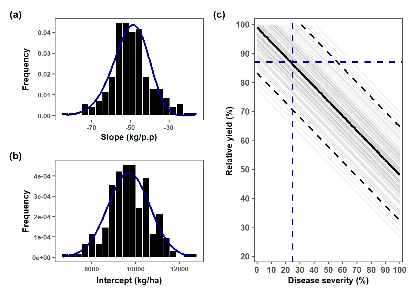

ggsave("fig/relative_parameters.png", bg = "white", dpi = 600,
       height = 4, width = 6)

Break-even probability

Framework simulation

NORTA function

gera.norm.bid.geral<-function(tamanho.amostra,correlacao,m1,m2,sigma1,sigma2)
{
  ro<-correlacao
  n<-tamanho.amostra
  x<-matrix(0,n,2)
  for (i in 1:n)
  {x[i,1]<-rnorm(1,m1,sigma1)
  x[i,2]<-rnorm(1,m2+ro*sigma1/sigma2*(x[i,1]-m1),sigma2*(sqrt(1-ro^2)))
  }
  return(x)
}

gc()

          used  (Mb) gc trigger  (Mb) max used  (Mb)
Ncells 2949079 157.5    4708747 251.5  4708747 251.5
Vcells 5853168  44.7   64697311 493.7 80871135 617.0

estria2 %>% 
  ggplot(aes(mean_sev))+
  geom_histogram(color= "white", fill = "black")+
  ggthemes::theme_few()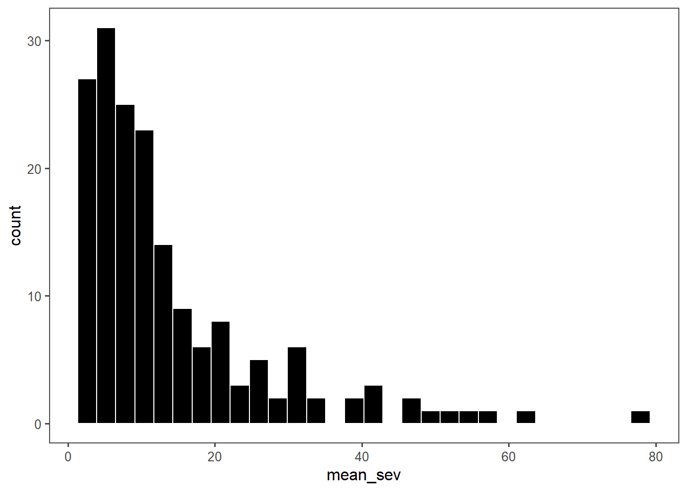

Severity

library(minpack.lm)
  
sev = simulated_data_lmer$sev
#sev = estria2$mean_sev
Fx_sev = environment(ecdf(sev))$y
x_sev = environment(ecdf(sev))$x/100

summary(nlsLM(Fx_sev ~ pbeta(x_sev, shape1, shape2, log = FALSE) ,
      start = c(shape1 = 1, shape2 = 1),
      control = nls.lm.control(maxiter = 100000)))

Formula: Fx_sev ~ pbeta(x_sev, shape1, shape2, log = FALSE)

Parameters:
        Estimate Std. Error t value Pr(>|t|)    
shape1 1.2041125  0.0005694    2115   <2e-16 ***
shape2 3.6414300  0.0020387    1786   <2e-16 ***
---
Signif. codes:  0 '***' 0.001 '**' 0.01 '*' 0.05 '.' 0.1 ' ' 1

Residual standard error: 0.004923 on 9998 degrees of freedom

Number of iterations to convergence: 7 
Achieved convergence tolerance: 1.49e-08

ks.test(Fx_sev,pbeta(x_sev,1.2041125,3.6414300))

    Asymptotic two-sample Kolmogorov-Smirnov test

data:  Fx_sev and pbeta(x_sev, 1.2041125, 3.64143)
D = 0.0111, p-value = 0.5689
alternative hypothesis: two-sided

plot(x_sev,Fx_sev)
curve(pbeta(x, 1.2041125,3.6414300),0,1, add = T)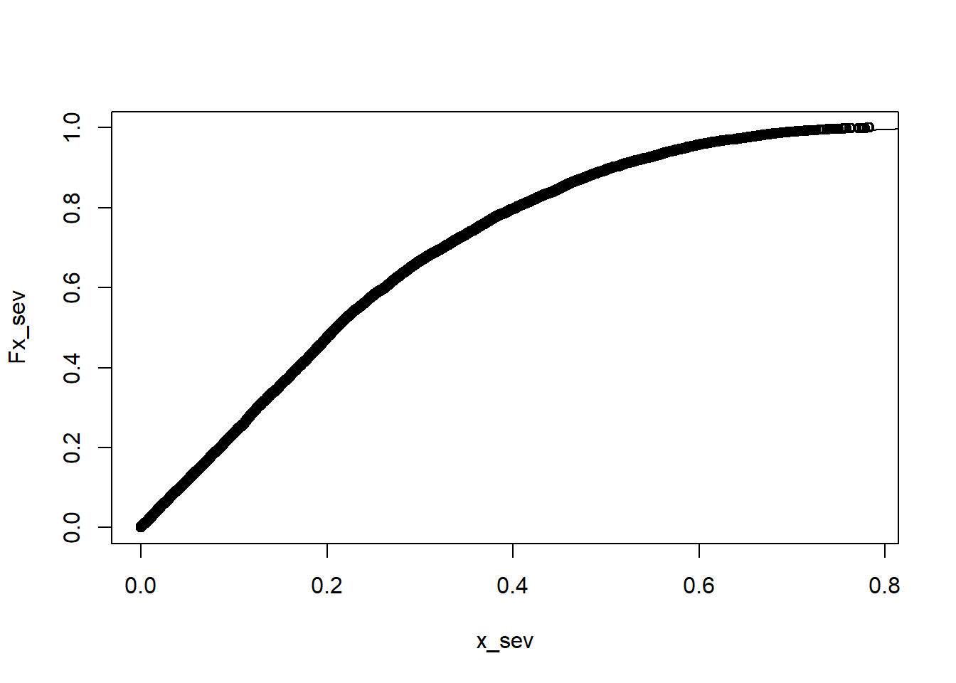

Intercept

intercept_bls = regression_trial_m
intercept_bls[,1] = NULL

mean_intercept = mean(intercept_bls$Intercept)
sd_intercept = sd(intercept_bls$Intercept)

plot(ecdf(intercept_bls$Intercept))
curve(pnorm(x, mean_intercept,sd_intercept), add = T, col = "red")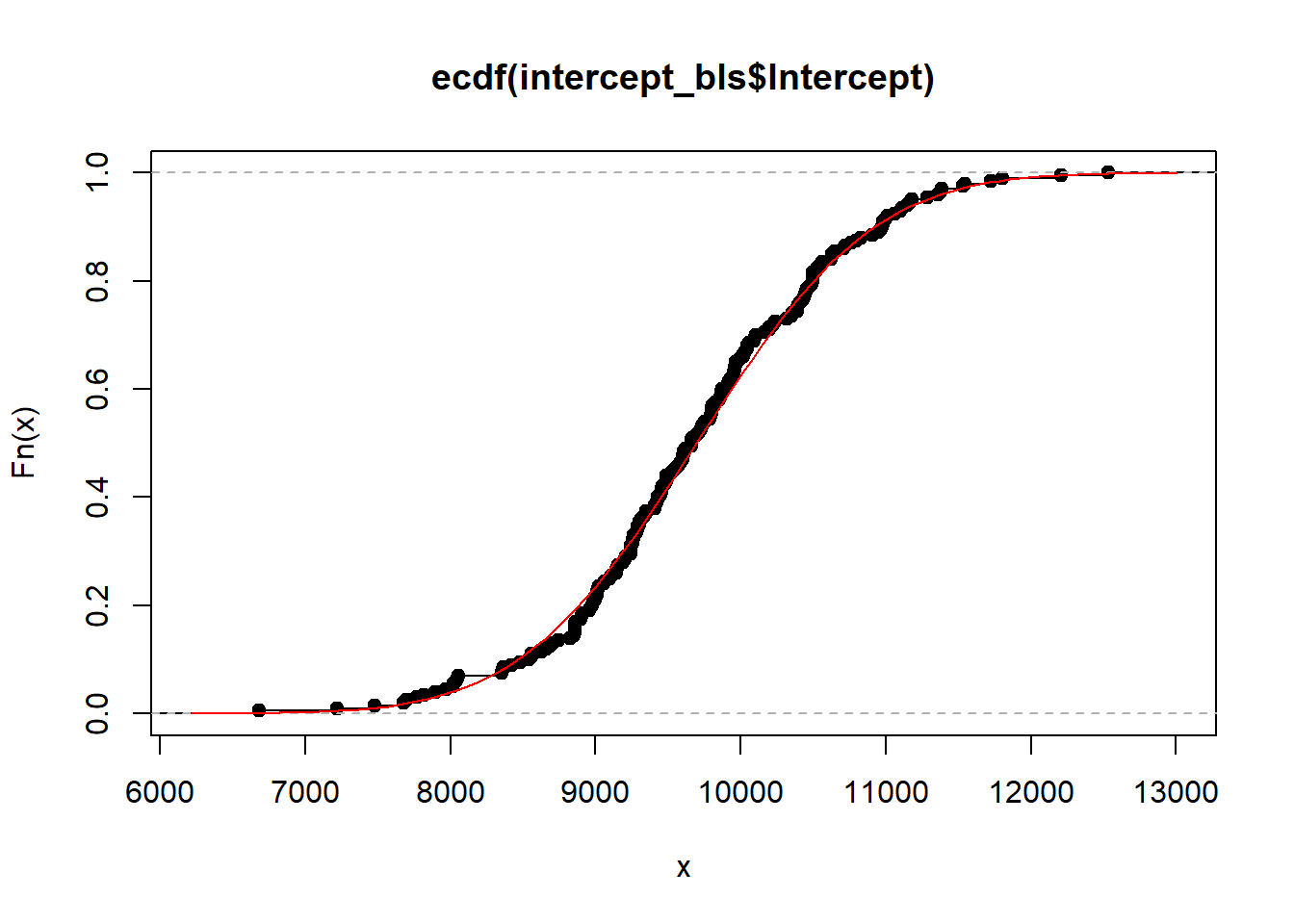

Fx_res_b0 = environment(ecdf(intercept_bls$Intercept))$y
x_res_b0= environment(ecdf(intercept_bls$Intercept))$x
ks.test(Fx_res_b0, pnorm(x_res_b0, mean(intercept_bls$Intercept), sd(intercept_bls$Intercept)))

    Asymptotic two-sample Kolmogorov-Smirnov test

data:  Fx_res_b0 and pnorm(x_res_b0, mean(intercept_bls$Intercept), sd(intercept_bls$Intercept))
D = 0.045, p-value = 0.9874
alternative hypothesis: two-sided

Slope

slope_bls = regression_trial_m
slope_bls[,2] = NULL
  

mean_slope = mean(slope_bls$Slope)
sd_slope = sd(slope_bls$Slope)

plot(ecdf(slope_bls$Slope))
curve(pnorm(x, mean_slope, sd_slope), add = T, col = "red")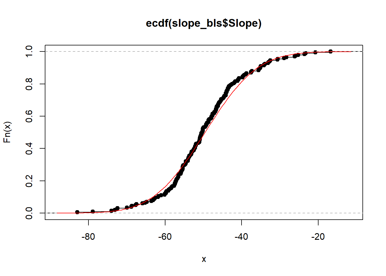

library(minpack.lm)
Fx =environment(ecdf(-slope_bls$Slope))$y
x = environment(ecdf(-slope_bls$Slope))$x

slope_reg = nlsLM(Fx ~ pgamma(x, shape, rate,log = FALSE) ,
      start = c(shape = 2.5, rate = 0.13),
      control = nls.lm.control(maxiter = 1024))
summary(slope_reg)

Formula: Fx ~ pgamma(x, shape, rate, log = FALSE)

Parameters:
      Estimate Std. Error t value Pr(>|t|)    
shape 29.25149    0.62746   46.62   <2e-16 ***
rate   0.58169    0.01255   46.37   <2e-16 ***
---
Signif. codes:  0 '***' 0.001 '**' 0.01 '*' 0.05 '.' 0.1 ' ' 1

Residual standard error: 0.02492 on 198 degrees of freedom

Number of iterations to convergence: 12 
Achieved convergence tolerance: 1.49e-08

shape = summary(slope_reg)$coef[1]
rate = summary(slope_reg)$coef[2]

Fx =environment(ecdf(-slope_bls$Slope))$y
x = environment(ecdf(-slope_bls$Slope))$x
ks.test(Fx, pgamma(x, shape, rate))

    Asymptotic two-sample Kolmogorov-Smirnov test

data:  Fx and pgamma(x, shape, rate)
D = 0.08, p-value = 0.5441
alternative hypothesis: two-sided

cor(regression_trial_m$Slope,regression_trial_m$Intercept)

[1] -0.1547164

j_res<-gera.norm.bid.geral(10000,0.15,0,0,1,1)

plot(j_res[,1],j_res[,2])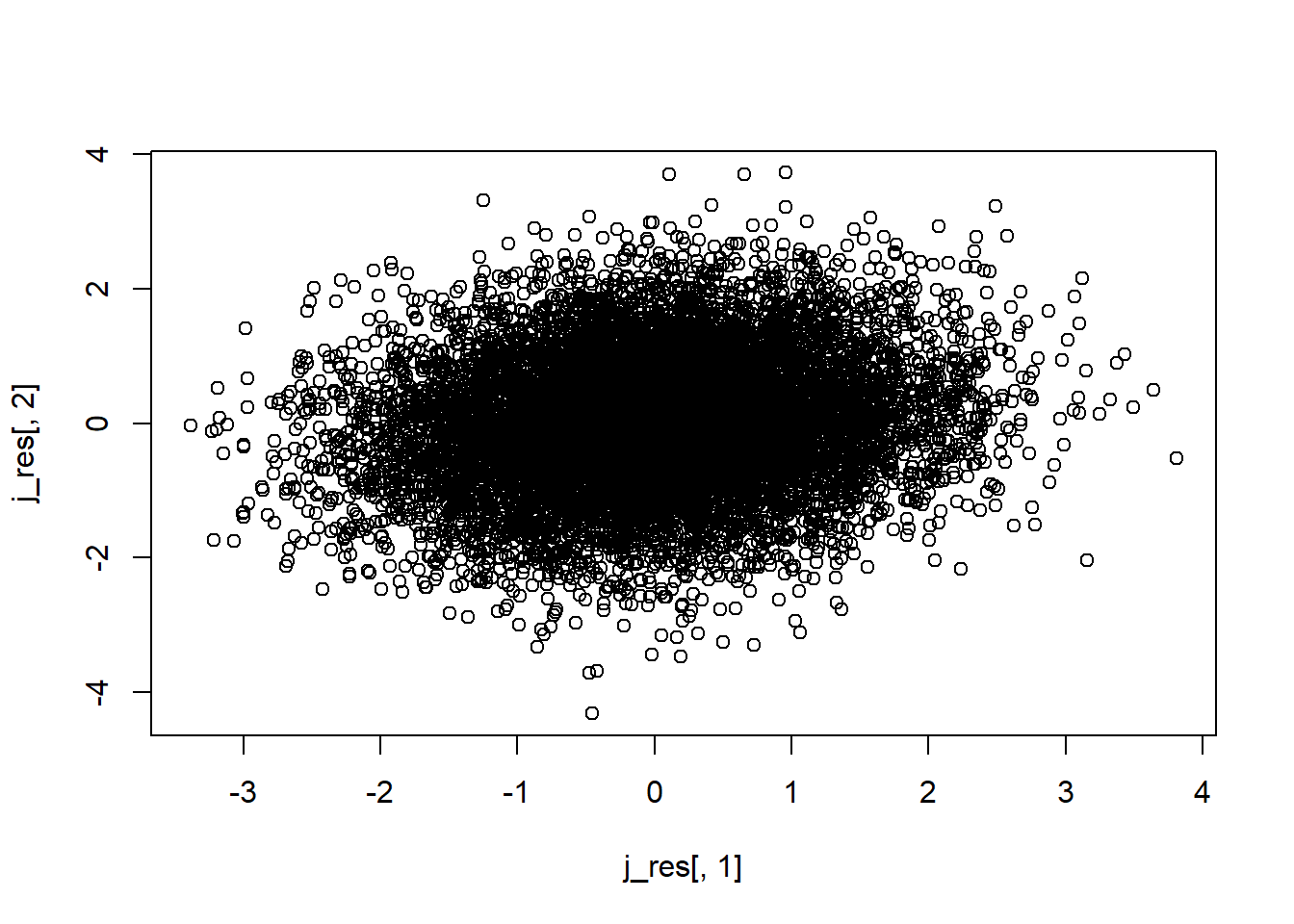

Corn price

corn = gsheet2tbl("https://docs.google.com/spreadsheets/d/1LcLVKb6bW7tVaiu6reLsT8sjFR1hwUcembZ7uxAoBP8/edit?usp=sharing") 

corn = corn %>%
  filter(state %in% c("PR")) %>% 
  filter(year <= 2019)

bls_price = corn %>%
  #filter(year <= 2019) %>%
  mutate(price = (price/60)/4)
bls_price

min(bls_price$price)

[1] 0.07679167

mean(bls_price$price)

[1] 0.1153426

mean(bls_price$price)

[1] 0.1153426

median(bls_price$price)

[1] 0.12

sd(bls_price$price)

[1] 0.0198195

bls_price %>% 
  ggplot(aes(price))+
  geom_histogram(fill = "steelblue", color = "white", bins = 10)+
 ggthemes::theme_few()+
  labs(x = "Soybean prince",
       y = "Frequency")+
  scale_x_continuous(breaks = seq(0,1,by=0.025))+
  theme(text = element_text(size = 12, face = "bold"),
        axis.title = element_text(size = 14, face = "bold"),
        legend.position = "none")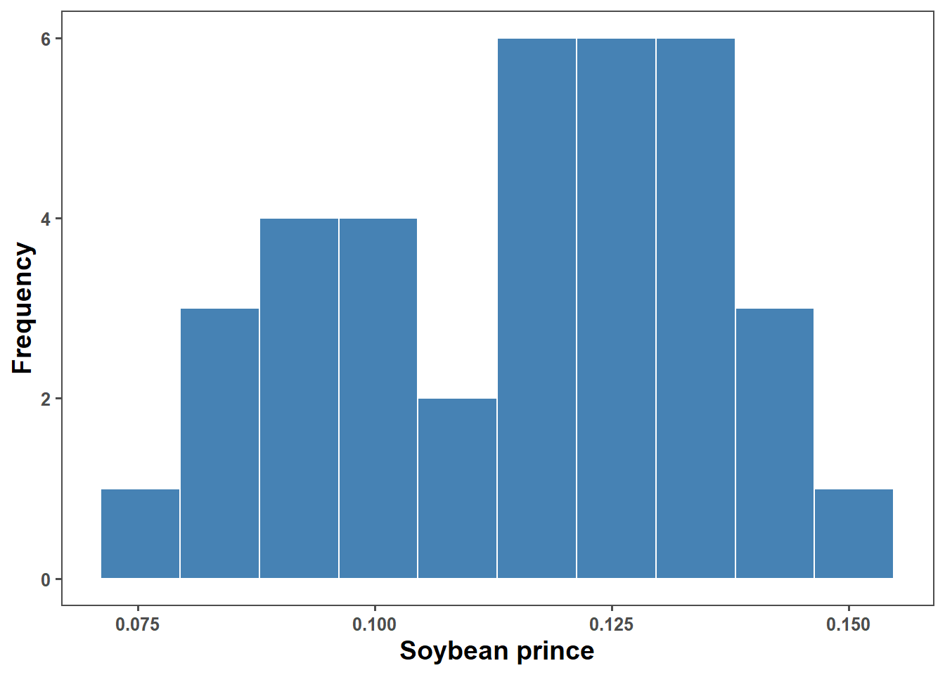

hist((bls_price$price), prob = T)
curve(dnorm(x, mean(bls_price$price), sd(bls_price$price)),0.15,0.35, add = T)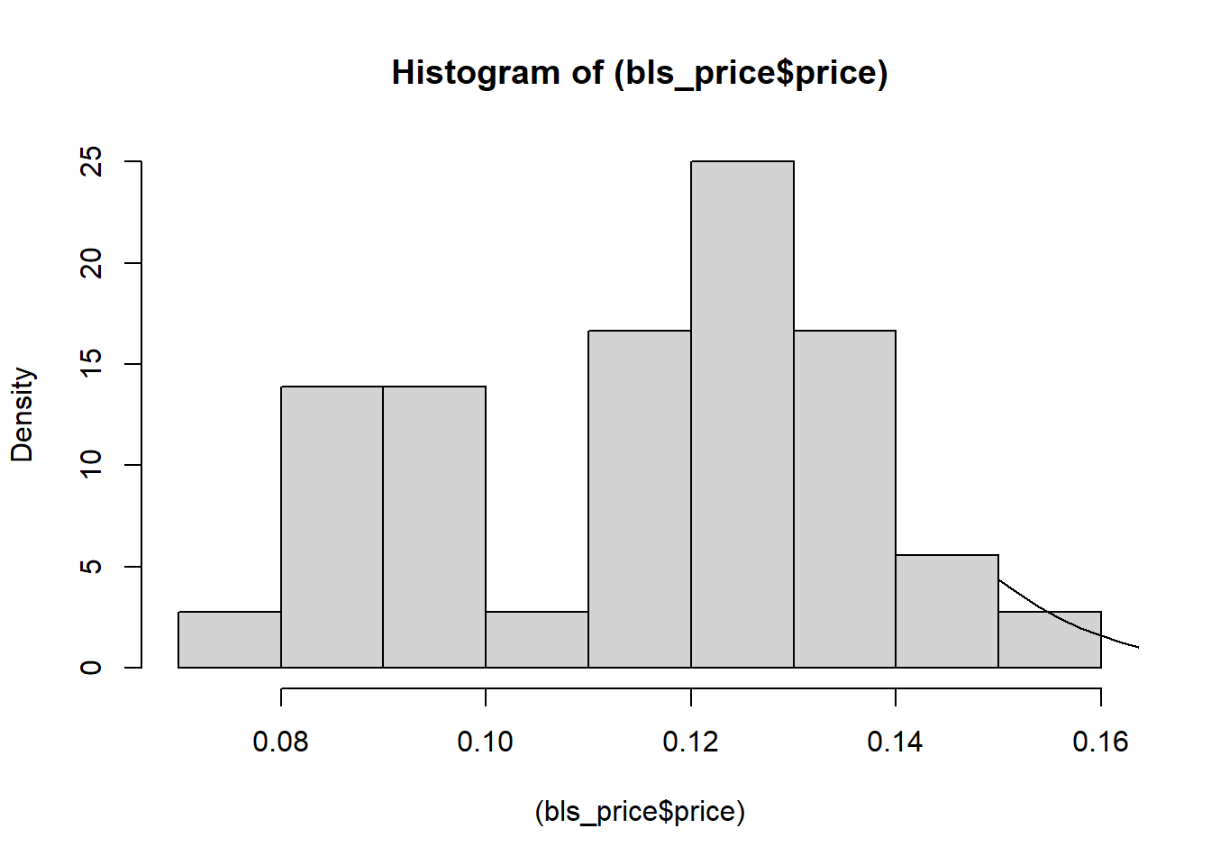

plot(ecdf(bls_price$price))
curve(pnorm(x, mean(bls_price$price), sd(bls_price$price)),0.2,0.35, add = T)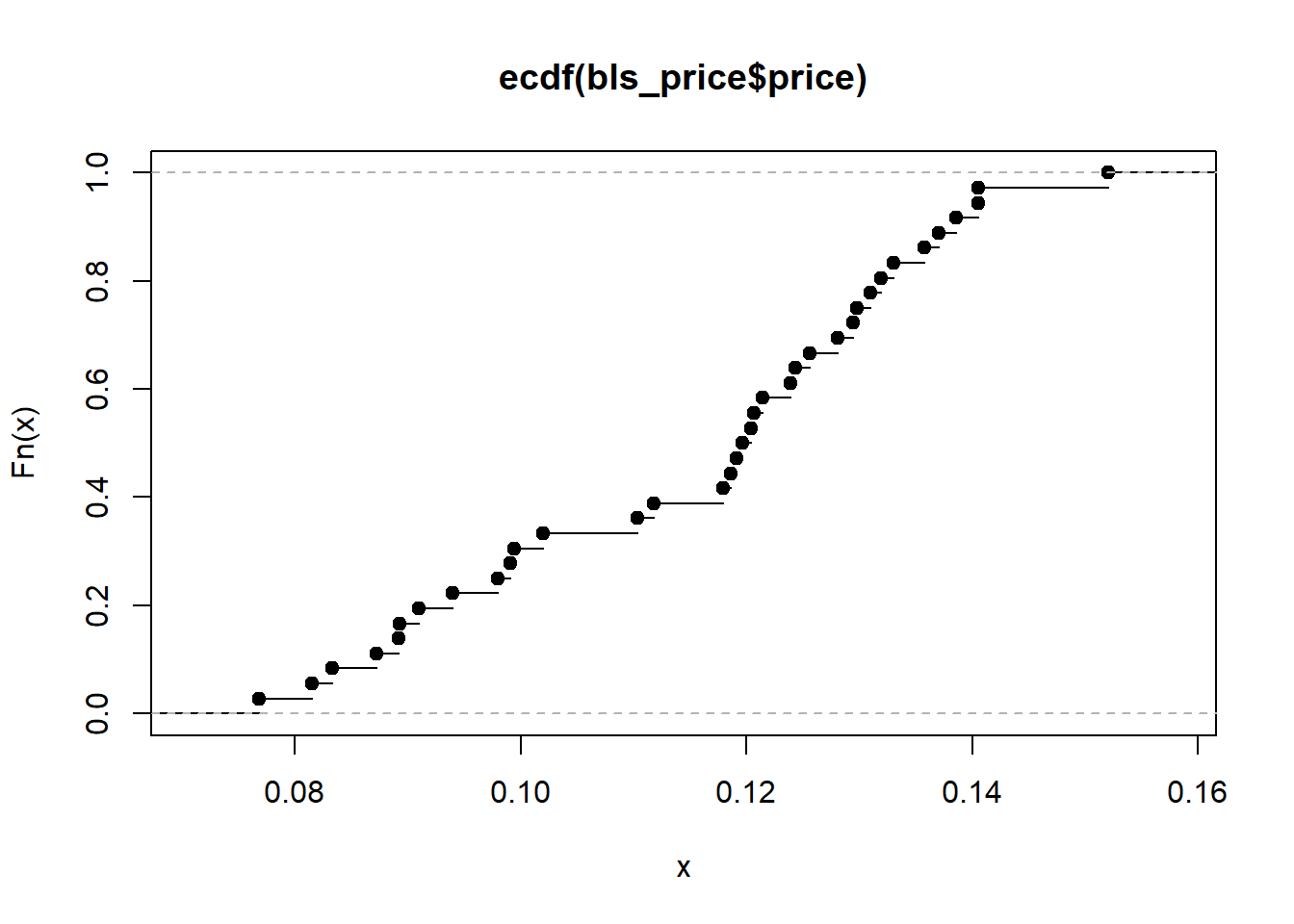

mean(bls_price$price)

[1] 0.1153426

median(bls_price$price)

[1] 0.12

shapiro.test(bls_price$price)

    Shapiro-Wilk normality test

data:  bls_price$price
W = 0.94849, p-value = 0.0937

Kolmogorov-Smirnov Test

Fx = environment(ecdf(bls_price$price))$y
x= environment(ecdf(bls_price$price))$x
ks.test(Fx, pnorm(x, mean(bls_price$price), sd(bls_price$price)))

    Exact two-sample Kolmogorov-Smirnov test

data:  Fx and pnorm(x, mean(bls_price$price), sd(bls_price$price))
D = 0.13889, p-value = 0.8849
alternative hypothesis: two-sided

plot(Fx, pnorm(x, mean(bls_price$price), sd(bls_price$price)))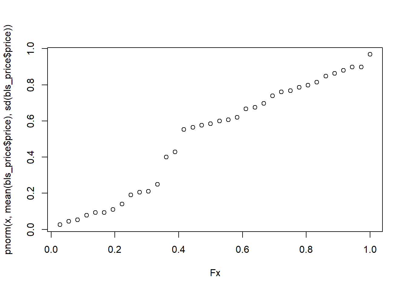

Vizualization

price_plot = bls_price %>% 
  ggplot(aes(price))+
 geom_histogram(aes(y = ..density..),bins = 10, color = "white", fill = "black")+ #"#1C8C20"
   #stat_function(fun=function(x) dnorm(x, mean(sbr_price$price), sd(sbr_price$price)), color= "black", size = 1.2)+
  ggthemes::theme_few()+
  labs(x="Soybean price (USD/kg)", y = "Frequency")+
  scale_x_continuous(breaks = seq(0,1,by=0.025))+
theme(text = element_text(size = 12, face = "bold"),
        axis.title = element_text(size = 14, face = "bold"),
        legend.position = "none")
price_plot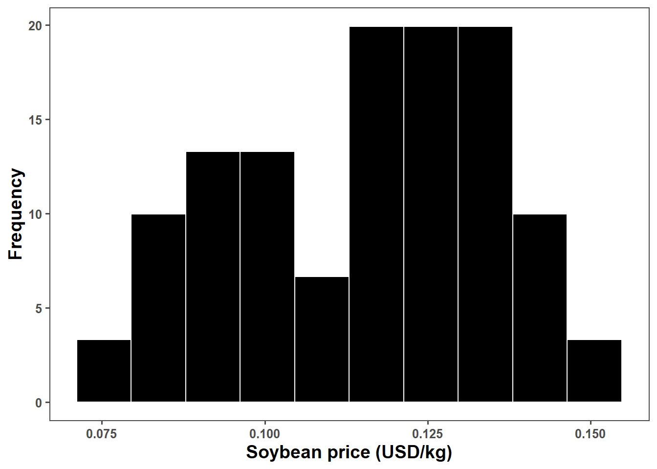

  ggsave("fig/soybean_price.png", bg = "white",
       dpi = 600, height = 5, width = 6)

Simulation

set.seed(1)
n=40000
lambda = seq(0,1, by=0.05)
fun_price = seq(-10, 260, by=15)
n_aplication = 1
operational_cost = 10  

comb_matrix = as.matrix(data.table::CJ(lambda,fun_price))
colnames(comb_matrix) = c("lambda","fun_price")
comb_matrix = cbind(comb_matrix,operational_cost, n_aplication)
C = comb_matrix[,"n_aplication"]*(comb_matrix[,"operational_cost"]+comb_matrix[,"fun_price"] )
comb_matrix = cbind(comb_matrix,C)

N = length(comb_matrix[,1])*n
big_one = matrix(0, ncol = 12, nrow =N)
big_one[,1] = rep(comb_matrix[,1],n)
big_one[,2] = rep(comb_matrix[,2],n)
big_one[,3] = rep(comb_matrix[,3],n)
big_one[,4] = rep(comb_matrix[,4],n)
big_one[,5] = rep(comb_matrix[,5],n)

set.seed(1)


sn = rbeta(N, 1.2041125,3.6414300)
sf = sn*(1-big_one[,1])

# simulating the coeficientes 


set.seed(1)
normal_correlated<-gera.norm.bid.geral(N,0.15,0,0,1,1)
b0_n = pnorm(normal_correlated[,2])
b1_n = pnorm(normal_correlated[,1])
b0 = qnorm(b0_n, mean_intercept,sd_intercept)
b1 = -qgamma(b1_n, shape, rate,)
rm(b0_n,b1_n,normal_correlated)


# Calculating the alha coeficient


alfa = (b1/b0)*100

# Calculating yield gain

## Moderate Resistant (MR)

yn  = b0 - (-alfa*b0*sn)
yf  = b0 - (-alfa*b0*sf)


# Simulating soybean price

set.seed(1)
soy_price = rnorm(N, mean(bls_price$price),sd(bls_price$price))

#income = yield_gain*soy_price # calculating the income

big_one[,6] = yn
big_one[,7] = yf
big_one[,8] = b1
big_one[,9] = b0
big_one[,10] = sn
big_one[,11] = sf
big_one[,12] = soy_price
colnames(big_one)  = c("lambda","fun_price","operational_cost","n_aplication","C","yn","yf",
                       "b1","b0","sn","sf","soy_price")

big_one_df = as.data.frame(big_one) %>% 
  filter(b0>=0) %>% 
  filter(yn>0) %>% 
  filter(alfa > -3 & alfa < 0) %>%
  mutate(yield_gain = yf-yn,
         yield_gain_perc = ((yf/yn)-1)*100,
         income = yield_gain*soy_price,#0.2
         CP = C/soy_price,#0.2
         profit = (income>=C)*1) %>% 
        filter(C <= 180) %>%
        filter(lambda >= 0.4) %>%
        filter(lambda <= 0.8)

gc()

#write_csv(big_one_df,"data/big_one_df.csv")
big_one_df = read_csv("data/big_one_df.csv")

sn = big_one_df %>% 
  ggplot(aes(sn))+
  geom_histogram(color = "white", fill = "steelblue", bins = 10, alpha= .5)+
  theme(text = element_text(face = "bold", size = 14),
        axis.title = element_text(face = "bold",size = 16))+
  labs(y = "Frequency",
       x = "BLS severity (%)")+
  ggthemes::theme_few()

gc()

           used  (Mb) gc trigger  (Mb) max used  (Mb)
Ncells  2957877 158.0    4708747 251.5  4708747 251.5
Vcells 85476209 652.2  125675078 958.9 85646906 653.5

b0_graphic = big_one_df %>% 
  ggplot(aes(b0))+
  geom_histogram(color = "white", fill = "steelblue", bins = 10, alpha= .5)+
   #scale_x_continuous(breaks = c(0,1000,2000,3000,4000,5000,6000,7000), limits = c(0, 7000))+
  theme(text = element_text(face = "bold", size = 14),
         axis.title = element_text(size = 16, face = "bold"))+
  labs(y = "Frequency",
       x = "Intercept (kg/ha)")+
  ggthemes::theme_few()

gc()

           used  (Mb) gc trigger  (Mb) max used  (Mb)
Ncells  2958594 158.1    4708747 251.5  4708747 251.5
Vcells 85478145 652.2  125675078 958.9 85646906 653.5

b1_graphic = big_one_df %>% 
  ggplot(aes(b1))+
  geom_histogram(color = "white", fill = "steelblue", bins = 10, alpha= .5)+
  #scale_x_continuous(breaks = c(-100,-90,-80,-70,-60,-50,-40,-30,-20,-10,0), limits = c(-100,0))+
  theme(text = element_text(face = "bold", size = 14),
         axis.title = element_text(size = 16, face = "bold"))+
  labs(y = "Frequency",
       x = "Slope (kg/p.p.)")+
  ggthemes::theme_few()

gc()

           used  (Mb) gc trigger  (Mb) max used  (Mb)
Ncells  2959325 158.1    4708747 251.5  4708747 251.5
Vcells 85480112 652.2  125675078 958.9 85646906 653.5

b1_graphic

alpha_graphic = big_one_df %>% 
    filter(C <= 180) %>%
  filter(lambda >= 0.4) %>%
  filter(lambda <= 0.8) %>%
  filter(C >= 60) %>%
  ggplot(aes(alfa))+
  geom_histogram(color = "white", fill = "black", bins = 10)+
  #scale_x_continuous(breaks = c(-2.0,-1.75,-1.50,-1.25,-1.00,-0.75,-0.50,-0.25,0.0), limits = c(-2.0,0.0))+
  theme(text = element_text(face = "bold", size = 14),
         axis.title = element_text(size = 16, face = "bold"))+
  labs(y = "Frequency",
       x = "Yield loss (%/p.p.)")+
  ggthemes::theme_few()

gc()

alpha_graphic

#alpha_res_graphic,alpha_m_sus_graphic,alpha_sus_graphic,
plot_grid(sn_res_graphic,b0_res_graphic,b1_res_graphic, ncol = 3,  labels = c("(a)", "(b)", "(c)"),label_x = -0.03)

ggsave("fig/simulated_variables.png", dpi = 1000, bg = "white",
       height = 8, width = 12)

heat <- big_one_df %>%
  filter(C <= 180) %>%
  filter(lambda >= 0.4) %>%
  filter(lambda <= 0.8) %>%
  filter(C >= 15) %>%
  group_by(lambda, C) %>%
  summarise(n = n(), sumn = sum(profit), prob = sumn / n) 

gc()

           used  (Mb) gc trigger   (Mb)  max used   (Mb)
Ncells  2959523 158.1    4708747  251.5   4708747  251.5
Vcells 85481175 652.2  261029279 1991.5 261024076 1991.5

heat_graphic = heat %>% 
  ggplot(aes(as.factor(lambda * 100), as.factor(C), fill = prob)) +
  geom_tile(size = 0.5, color = "white") +
  scale_fill_viridis_b(option = "D", direction = -1) +
  scale_color_manual(values = c("#E60E00", "#55E344")) +
  guides(color = guide_legend(override.aes = list(size = 2))) +
  labs(x = "Fungicide efficacy (%)",
       y = "Fungicide + Application cost ($)",
       fill = "Pr(I \u2265 C)",
       color = "") +
 # facet_wrap(vars(class, class2)) +
  ggthemes::theme_few()+
  theme(strip.text = element_text(face = "bold", size = 14),
        text = element_text(face = "bold", size = 14))


gc()

           used  (Mb) gc trigger   (Mb)  max used   (Mb)
Ncells  2962435 158.3    4708747  251.5   4708747  251.5
Vcells 85486263 652.3  261029279 1991.5 261024076 1991.5

big = big_one_df %>%
   mutate(class = case_when(sn > 0.25 ~ "High severity",
                           sn <= 0.25 ~"Low severity"))

class <- big %>%
  filter(C <= 105) %>%
  filter(lambda >= 0.4) %>%
  filter(lambda <= 0.8) %>%
  filter(C >= 15) %>%
  group_by(lambda, C, class) %>%
  summarise(n = n(), sumn = sum(profit), prob = sumn / n, .groups = 'drop') %>%
  ungroup()  

gc()

           used  (Mb) gc trigger   (Mb)  max used   (Mb)
Ncells  2962483 158.3    4708747  251.5   4708747  251.5
Vcells 90167142 688.0  261029279 1991.5 261024076 1991.5

library(viridis)
heat_graphic = class %>% 
  filter(!is.na(class)) %>% 
  ggplot( aes(as.factor(lambda * 100), as.factor(C), fill = prob)) +
  geom_tile(size = 0.5, color = "white") +
  #geom_text(aes(label = paste(round(prob, 2), sep = "")),
   # size = 4, colour = "white")+
  scale_fill_viridis_b(option = "E", direction =  -1)+
  #scale_fill_viridis(discrete = T, option = "E") +
  guides(color = guide_legend(override.aes = list(size = 2))) +
  labs(x = "Treatment efficacy (%)",
       y = "Treatment cost (USD/ha)",
       fill = "Pr(I \u2265 C)",
       color = "") +
  facet_wrap(vars(class), ncol =1) +
  ggthemes::theme_few()+
  theme(strip.text = element_text(face = "bold", size = 14),
        text = element_text(face = "bold", size = 14),
        legend.position = "right")

gc()

           used  (Mb) gc trigger   (Mb)  max used   (Mb)
Ncells  2963942 158.3    4708747  251.5   4708747  251.5
Vcells 90170579 688.0  261029279 1991.5 261024076 1991.5

low_class = class %>% 
  filter(class == "Low severity")

min(low_class$prob)

[1] 0.0002628466

max(low_class$prob)

[1] 0.8714784

mean(low_class$prob)

[1] 0.3308383

low_class %>% 
  filter(C <= 15)

high_class = class %>% 
  filter(class == "High severity")

min(high_class$prob)

[1] 0.3460665

max(high_class$prob)

[1] 1

mean(high_class$prob)

[1] 0.9033795

overall = big %>%
  filter(C <= 105) %>%
  filter(C >= 15) %>%
  #mutate(sev_class = " Overall") %>% 
  dplyr::group_by(lambda,class) %>% 
  summarise(yield_gain_median = median(yield_gain),
            yield_gain_mean = mean(yield_gain),
            up_95 = quantile(yield_gain, 0.975),
            low_95 = quantile(yield_gain, 0.025),
            up_75 = quantile(yield_gain, 0.75),
            low_75 = quantile(yield_gain, 0.25)) 

 gain_graphic = overall %>% 
  ggplot(aes(lambda*100,yield_gain_mean))+
  geom_line(aes(lambda*100, low_95),
              linetype = 2,
            size = 1,
            fill = NA, color = "black")+
  geom_line(aes(lambda*100, up_95),
              linetype = 2,
            size = 1,
          fill = NA,color = "black")+
  geom_line(size = 1.4, aes(lambda*100,yield_gain_median), color = "#ffc425")+
   #scale_y_continuous(breaks = c(0, 500, 1000, 1500,2000,
    #                             2500, 3000), 
     #                 limits = c(0, 3000))+
   #scale_x_continuous(breaks = c(40,50,60,70,80), limits = c(40, 80))+
  #scale_color_viridis_d()+
  #scale_color_manual(values = c('steelblue', '#9ccb86', 'darkred'))+
  ggthemes::theme_few()+
  facet_wrap(~class, ncol = 1)+
  #facet_wrap(~class+class2)+
  labs(x = "Treatment efficacy (%)",
       y = "Yield difference (kg/ha)",
       color = "Tolerance level", 
       linetype = "", fill = "")+
  theme(text = element_text(face = "bold", size = 14),
        strip.text = element_text(size = 14),
        legend.position = "top")

library(cowplot)

(gain_graphic+heat_graphic) +
  plot_annotation(tag_levels = "a", tag_prefix = "(", tag_suffix = ")")&
  theme(plot.tag = element_text(face = "bold", size = 16))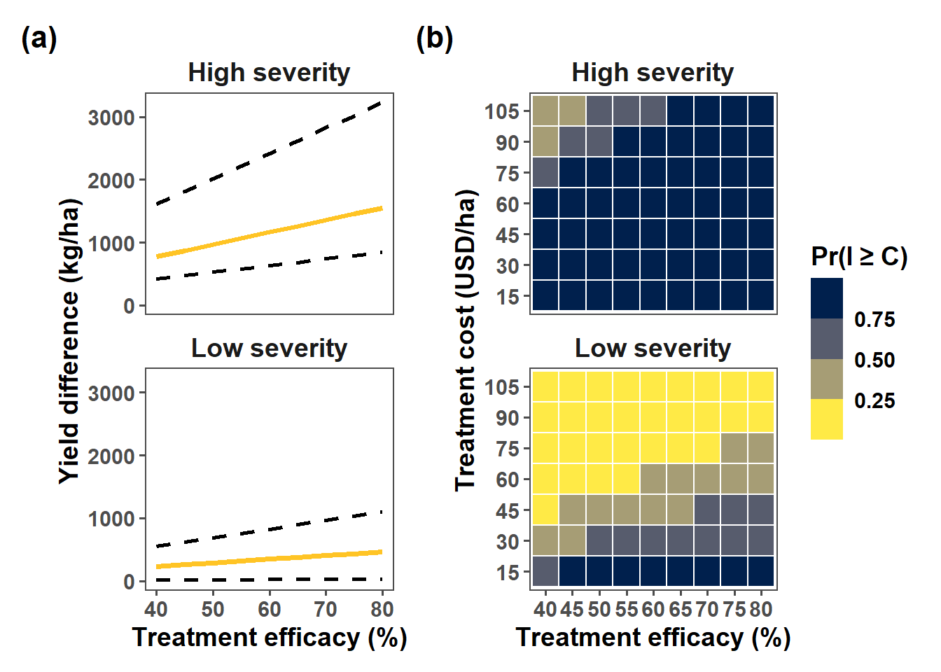

ggsave("fig/break-even_gain.png", dpi = 600, bg = "white",
       width = 8, height = 6)